import ibis
import pandas as pd
from ibis import _
archive = ibis.read_parquet("https://raw.githubusercontent.com/aeturrell/real-time-data/realtimedata.parquet")Accessing the data
Downloading in bulk or running queries
The archive consists of a single parquet file (currently 2.3 MB.) The file is published as part of the site. You can download it, or point a query tool at its web address and read it from there.
Query the data without downloading the file
We recommend DuckDB for querying cuts of the data. DuckDB is a free database query engine that runs on your own computer and can read a parquet file from a web address.
The example query below asks for every value of UK GDP growth in the second quarter of 2020:
SELECT vintage_date::DATE AS published, value
FROM 'https://raw.githubusercontent.com/aeturrell/real-time-data/realtimedata.parquet'
WHERE series_id = 'IHYQ' AND reference_period = '2020Q2'
ORDER BY vintage_date
Another example: list every series, with its name and the dates of its first and latest publications:
SELECT
    series_id,
    any_value(title) AS title,
    min(vintage_date)::DATE AS first_published,
    max(vintage_date)::DATE AS latest_published
FROM 'https://raw.githubusercontent.com/aeturrell/real-time-data/realtimedata.parquet'
GROUP BY series_id
ORDER BY series_id
To run a query from the command line, install DuckDB and, if using from the command line, pass the query to it in quotes:
duckdb -c "
  SELECT vintage_date::DATE AS published, value
  FROM 'https://raw.githubusercontent.com/aeturrell/real-time-data/realtimedata.parquet'
  WHERE series_id = 'IHYQ' AND reference_period = '2020Q2'
  ORDER BY vintage_date"
You can also paste either query into DuckDB’s browser shell without installing anything. It works because the file’s host sets CORS (cross-origin resource sharing), a permission that lets web pages on other sites read the file.
Bulk download the file
curl -O https://raw.githubusercontent.com/aeturrell/real-time-data/realtimedata.parquetExplore the data
DuckDB also comes with a notebook-style interface, which is an easy way to browse the archive. It needs DuckDB 1.2.1 or later. If you already have duckdb, start the user interface with:
duckdb -uiThis opens the interface in your browser, installing the extension it needs on first run. In a notebook cell, make a view (a saved query you can treat as a table) of the file:
CREATE VIEW realtime AS
SELECT * FROM 'https://raw.githubusercontent.com/aeturrell/real-time-data/realtimedata.parquet'
Click realtime in the list on the left to see each column’s type and a summary of its values, then write queries against it in further cells. The DuckDB UI documentation covers the options, and the announcement of DuckDB UI gives a tour of its features.
Use the data from Python
The rest of this page works from Python using Ibis, which writes queries that are executed by DuckDB. You’ll need DuckDB and Ibis in your Python installation to run this. Run uv add 'ibis-framework[duckdb]' pandas duckdb.
Queries are ordinary Python code. Every example can be copied and run as it is.
In these examples, _ stands for the table at that step of the query, so _.value means its value column.
See the numbers as they stood on a past date
Here is the 2008 recession, as it looked at the end of January 2009 and as it looks now:
KNOWN_ON = "2009-01-31"

known_then = _.vintage_date <= ibis.timestamp(KNOWN_ON)

recession = (
    archive.filter(
        _.series_id == "IHYQ",
        _.frequency == "Q",
        _.reference_period.between("2008Q1", "2008Q4"),
    )
    .group_by(quarter=_.reference_period)
    .agg(
        growth_then=_.value.argmax(_.vintage_date, where=known_then),
        growth_now=_.value.argmax(_.vintage_date),
    )
    .order_by("quarter")
    .to_pandas()
)| Quarter | Growth known in January 2009 (%) | Growth known now (%) |
|---|---|---|
| 2008Q1 | 0.4 | 0.4 |
| 2008Q2 | 0.0 | -0.5 |
| 2008Q3 | -0.6 | -1.5 |
| 2008Q4 | -1.5 | -2.1 |
Adding up the four quarters gives a rough sense of the difference: -1.7 percentage points as seen at the time, and -3.7 now. Anyone judging policy decisions from that winter should use the first column, because that is what people had in front of them.
Examples
These are just illustrative.
Follow a revision: unemployment
Unemployment rates are revised less than GDP growth, but they do change, sometimes in ways that alter the story. In October 2023 ONS stopped publishing its usual Labour Force Survey estimates, because too few people were responding. The survey returned in February 2024, reweighted to new population figures, and the data were reweighted again in December 2024.
This query collects each value of the unemployment rate (MGSX) with its publication date. The rates are rolling three-month figures, stored against the month each window ends.
UNEMPLOYMENT_FROM = "2021-01"
UNEMPLOYMENT_TO = "2024-06"

unemployment = (
    archive.filter(
        _.series_id == "MGSX",
        _.frequency == "M",
        _.reference_period.between(UNEMPLOYMENT_FROM, UNEMPLOYMENT_TO),
    )
    .select(month=_.reference_period, vintage_date=_.vintage_date, value=_.value)
    .order_by("vintage_date")
    .to_pandas()
)


def unemployment_known_on(date: str) -> pd.Series:
    """Rebuilds the unemployment rate as it stood on a given date.

    Args:
        date: The date of interest.

    Returns:
        The latest rate known that day, for each month.
    """
    known = unemployment.loc[unemployment["vintage_date"] <= date]
    return known.groupby("month")["value"].last().sort_index()


before_pause = unemployment_known_on("2023-09-12")
after_return = unemployment_known_on("2024-02-13")
latest = unemployment.groupby("month")["value"].last().sort_index()
first_estimates = unemployment.groupby("month")["value"].first().sort_index()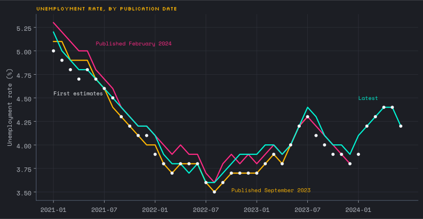
The February 2024 figures raised some earlier rates. For 2021-01, for example, the rate went from 5.1% to 5.3%. The later reweighting rewound some of that.
Compare how much series get revised
Because all series share one format, a single query can compare them. This takes each period’s first published value and its latest value, then measures the average gap. It leaves out history rows, because for those the archive does not hold the true first estimate. Recent periods have had less time to be revised, so these averages slightly understate the eventual gap.
QUARTERLY_SERIES = ["IHYQ", "KG7P"]
MONTHLY_SERIES = ["ECYX", "IOP_MOM", "RSI_MOM", "MGSX"]

estimates = (
    archive.filter(
        (_.series_id.isin(QUARTERLY_SERIES) & (_.frequency == "Q"))
        | (_.series_id.isin(MONTHLY_SERIES) & (_.frequency == "M"))
    )
    .group_by(["series_id", "reference_period"])
    .agg(
        title=_.title.arbitrary(),
        first_estimate=_.value.argmin(_.vintage_date),
        latest_estimate=_.value.argmax(_.vintage_date),
        first_release_type=_.release_type.argmin(_.vintage_date),
    )
)

revision_sizes = (
    estimates.filter(_.first_release_type == "first")
    .mutate(revision=(_.latest_estimate - _.first_estimate).abs())
    .group_by("series_id")
    .agg(
        title=_.title.arbitrary(),
        periods=_.count(),
        average_revision=_.revision.mean(),
        largest_revision=_.revision.max(),
    )
    .order_by(ibis.desc("average_revision"))
    .to_pandas()
)| Series | Title | Periods | Average revision (points) | Largest revision (points) |
|---|---|---|---|---|
| KG7P | Business investment quarter-on-quarter growth, CVM SA | 115 | 3.75 | 36.80 |
| IOP_MOM | Index of Production month-on-month growth | 344 | 0.69 | 4.10 |
| RSI_MOM | Retail Sales Index month-on-month growth | 345 | 0.56 | 4.10 |
| IHYQ | GDP quarter-on-quarter growth, chained volume measures, seasonally adjusted | 139 | 0.32 | 2.20 |
| ECYX | Gross Value Added - Monthly (period on period growth) :CVM SA | 111 | 0.24 | 1.50 |
| MGSX | UK unemployment rate, aged 16 and over | 333 | 0.04 | 0.30 |
Trace a value back to its source
Every row records where the value came from, when it was fetched and a SHA-256 fingerprint of the original file. You can use the fingerprint to check that a copy of the file is the one used here.
provenance = (
    archive.filter(
        _.series_id == "IHYQ",
        _.reference_period == "2020Q2",
        _.release_type == "first",
    )
    .select(
        _.value,
        published=_.vintage_date,
        source_url=_.source_url,
        retrieved=_.retrieved_at,
        content_sha256=_.content_sha256,
    )
    .to_pandas()
)
The first estimate of -20.4% was published on 12 August 2020. It came from this page on the ONS website, and the fingerprint of the data behind it begins 81011ecd5684.
An example nowcasting query
Of course, a major use case of real-time data is nowcasting. Below is an example that pulls quarterly GDP growth, monthly GDP, production, services, retail sales, unemployment, CPI inflation, and a business survey. All are growth rates, rates or scores, so their units do not shift between publications.
NOWCASTING_SERIES = {
    "IHYQ": "Quarterly GDP growth",
    "ECYX": "Monthly GDP growth",
    "IOP_MOM": "Production growth",
    "IOS_MOM": "Services growth",
    "RSI_MOM": "Retail sales growth",
    "MGSX": "Unemployment rate",
    "D7G7": "CPI inflation",
    "AGENTS_CONSUMER_SERVICES_VALUES": "Agents' consumer services score",
}

quarterly_or_monthly = (_.series_id == "IHYQ").ifelse("Q", "M")

nowcasting_data = (
    archive.filter(
        _.series_id.isin(list(NOWCASTING_SERIES)),
        _.frequency == quarterly_or_monthly,
    )
    .select("vintage_date", "reference_period", "series_id", "value")
    .order_by(["vintage_date", "series_id", "reference_period"])
    .to_pandas()
)

nowcasting_data.head()| vintage_date | reference_period | series_id | value | |
|---|---|---|---|---|
| 0 | 1992-05-31 | 1992Q1 | IHYQ | -0.6 |
| 1 | 1992-06-30 | 1992Q1 | IHYQ | -0.5 |
| 2 | 1992-08-31 | 1992Q2 | IHYQ | -0.1 |
| 3 | 1992-09-30 | 1992Q1 | IHYQ | -0.4 |
| 4 | 1992-11-30 | 1992Q3 | IHYQ | 0.0 |
Those are the oldest rows, and .tail() gives the newest. To see what a model would have had on any date, keep the rows published by then and take the newest value for each series and period.
Next, let’s pick a quarter and follow the data arriving between the day it began and the day of its first GDP estimate being released:
CHOSEN_QUARTER = pd.Period("2025Q3", "Q")

first_gdp_estimate_date = nowcasting_data.loc[
    (nowcasting_data["series_id"] == "IHYQ")
    & (nowcasting_data["reference_period"] == str(CHOSEN_QUARTER)),
    "vintage_date",
].min()
months_in_quarter = pd.period_range(CHOSEN_QUARTER.start_time, CHOSEN_QUARTER.end_time, freq="M")

quarter_rows = nowcasting_data.loc[
    nowcasting_data["vintage_date"].between(CHOSEN_QUARTER.start_time, first_gdp_estimate_date)
].copy()
quarter_rows["about_chosen_quarter"] = quarter_rows["reference_period"].isin(
    [str(month) for month in months_in_quarter] + [str(CHOSEN_QUARTER)]
)
quarter_rows["chosen_quarter_period"] = quarter_rows["reference_period"].where(
    quarter_rows["about_chosen_quarter"], other=""
)

releases = (
    quarter_rows.groupby(["series_id", "vintage_date"])
    .agg(
        rows=("value", "size"),
        about_chosen_quarter=("about_chosen_quarter", "any"),
        newest_period=("chosen_quarter_period", "max"),
    )
    .reset_index()
)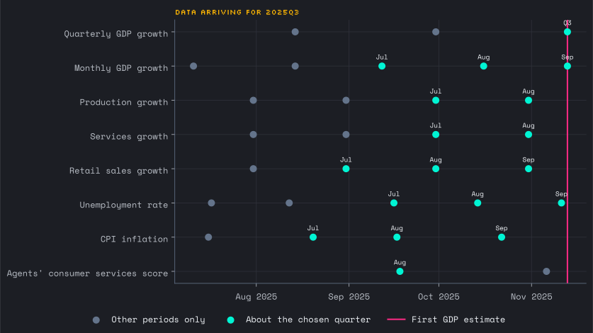
The first GDP estimate came on 13 November 2025. The earliest signal about the quarter in this set was CPI inflation, 85 days before that. A nowcast made partway through the quarter therefore has some series with figures for it and others that stop a month or two earlier. This uneven edge is what nowcasting models have to handle, and it is only visible with publication dates. Series can also skip a period: the archive holds no Agents’ score for September 2025, and that score’s dates are the latest it could have appeared, not exact days.
Do business surveys lead GDP?
Surveys of firms, often called soft data, come out sooner than official GDP. They often provide a useful early signal.
This example uses two Bank of England Agents’ scores, for consumer goods and consumer services, because they measure activity and have been public since 2006. Each is put on a common scale by subtracting its mean (\(\mu\)) and dividing by its standard deviation (\(\sigma\)):
\[ z = \frac{x - \mu}{\sigma} \]
The index is the average of the two over the latest three months.
For each quarter’s GDP release, the code keeps only the rows published before that day, so nothing from the future leaks in.
SURVEY_SERIES = ["AGENTS_CONSUMER_GOODS_VALUES", "AGENTS_CONSUMER_SERVICES_VALUES"]
RECENT_MONTHS = 3

survey_rows = (
    archive.filter(_.series_id.isin(SURVEY_SERIES))
    .select("series_id", "reference_period", "vintage_date", "value")
    .to_pandas()
)

gdp = (
    archive.filter(_.series_id == "IHYQ", _.frequency == "Q")
    .group_by(quarter=_.reference_period)
    .agg(
        first_estimate=_.value.argmin(_.vintage_date),
        latest_estimate=_.value.argmax(_.vintage_date),
        first_published=_.vintage_date.min(),
        first_release_type=_.release_type.argmin(_.vintage_date),
    )
    .filter(_.first_release_type == "first")
    .drop("first_release_type")
    .order_by("quarter")
    .to_pandas()
)
gdp.index = pd.PeriodIndex(gdp.pop("quarter"), freq="Q")
gdp = gdp.loc[gdp["first_published"] > survey_rows["vintage_date"].min()]


def survey_index_before(date: pd.Timestamp) -> float:
    """Builds the survey index from rows published before a given date.

    Args:
        date: The date of interest.

    Returns:
        The average standardised score over the latest months.
    """
    published = survey_rows.loc[survey_rows["vintage_date"] < date]
    scores = published.pivot_table(index="reference_period", columns="series_id", values="value")
    standardised = (scores - scores.mean()) / scores.std()
    return standardised.tail(RECENT_MONTHS).mean(axis=None)


gdp["survey_index"] = gdp["first_published"].map(survey_index_before)
The survey_index for a given quarter is what you could have worked out on the day before that quarter’s first GDP estimate. It is compared with GDP growth in that quarter and the following ones. As a benchmark, the last column uses that day’s first estimate of GDP instead of the survey index. (The pandemic and quarters from 2024 are left out.)
PANDEMIC_QUARTERS = pd.period_range("2020Q1", "2021Q4", freq="Q")
SETTLED_BEFORE = pd.Period("2024Q1", "Q")
EARLIEST_QUARTER = gdp.index.min()
RECENT_START = pd.Period("2016Q1", "Q")
QUARTERS_AHEAD = range(4)


def correlations_ahead(
    quarters_ahead: int,
    start: pd.Period = EARLIEST_QUARTER,
    leave_out_pandemic: bool = True,
) -> dict[str, float | int]:
    """Measures how closely the survey index tracks GDP growth some quarters ahead.

    Args:
        quarters_ahead: How many quarters after the survey index to look.
        start: The earliest quarter of the survey index to use.
        leave_out_pandemic: Whether to drop pairs with either quarter in the pandemic.

    Returns:
        The correlations with the first and latest estimates, the benchmark
        correlation and the number of quarters compared.
    """
    pairs = gdp.assign(
        first_ahead=gdp["first_estimate"].shift(-quarters_ahead),
        latest_ahead=gdp["latest_estimate"].shift(-quarters_ahead),
    ).dropna()
    target_quarters = pairs.index + quarters_ahead
    keep = (target_quarters < SETTLED_BEFORE) & (pairs.index >= start)
    if leave_out_pandemic:
        keep = keep & ~pairs.index.isin(PANDEMIC_QUARTERS) & ~target_quarters.isin(PANDEMIC_QUARTERS)
    kept = pairs.loc[keep]
    return {
        "quarters_ahead": quarters_ahead,
        "with_first": kept["survey_index"].corr(kept["first_ahead"]),
        "with_latest": kept["survey_index"].corr(kept["latest_ahead"]),
        "gdp_alone": kept["first_estimate"].corr(kept["first_ahead"]),
        "quarters_compared": len(kept),
    }


correlations = pd.DataFrame([correlations_ahead(quarters) for quarters in QUARTERS_AHEAD])| Quarters ahead | Survey index and first estimate | Survey index and latest estimate | First GDP estimate alone | Quarters compared |
|---|---|---|---|---|
| 0 | 0.53 | 0.62 | n/a | 65 |
| 1 | 0.52 | 0.55 | 0.58 | 63 |
| 2 | 0.46 | 0.38 | 0.44 | 61 |
| 3 | 0.33 | 0.18 | 0.20 | 59 |
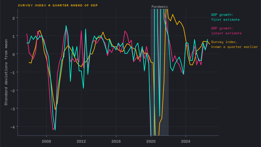
The survey index gives a modest early signal: one quarter ahead, its correlation with the first estimate is 0.52. The index pulls ahead three quarters out.