Introduction
In this chapter, you will learn a consistent way to organise your data in Python using the principle known as tidy data. Tidy data is not appropriate for everything, but for a lot of analysis and a lot of tabular data it will be what you need. Getting your data into this format requires some work up front, but that work pays off in the long term. Once you have tidy data, you will spend much less time munging data from one representation to another, allowing you to spend more time on the data questions you care about.
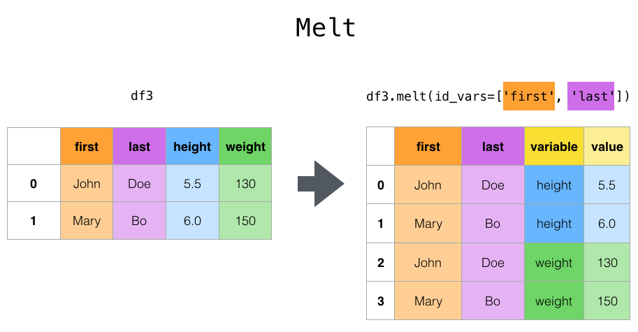
In this chapter, you’ll first learn the definition of tidy data and see it applied to simple toy dataset. Then we’ll dive into the main tool you’ll use for tidying data: melting. Melting allows you to change the form of your data, without changing any of the values. We’ll finish up with a discussion of usefully untidy data, and how you can create it if needed.
If you particularly enjoy this chapter and want to learn more about the underlying theory, you can learn more in the Tidy Data paper published in the Journal of Statistical Software.
Prerequisites
This chapter will use the pandas data analysis package.
Tidy Data
There are three interrelated features that make a dataset tidy:
- Each variable is a column; each column is a variable.
- Each observation is row; each row is an observation.
- Each value is a cell; each cell is a single value.
The figure below shows this:

Why ensure that your data is tidy? There are two main advantages:
There’s a general advantage to picking one consistent way of storing data. If you have a consistent data structure, it’s easier to learn the tools that work with it because they have an underlying uniformity. Some tools, for example data visualisation package seaborn, are designed with tidy data in mind.
There’s a specific advantage to placing variables in columns because it allows you to take advantage of pandas’ vectorised operations (operations that are more efficient).
Tidy data aren’t going to be appropriate every time and in every case, but they’re a really, really good default for tabular data. Once you use it as your default, it’s easier to think about how to perform subsequent operations.
Having said that tidy data are great, they are, but one of pandas’ advantages relative to other data analysis libraries is that it isn’t too tied to tidy data and can navigate awkward non-tidy data manipulation tasks happily too.
There are two common problems you find in data that are ingested that make them not tidy:
- A variable might be spread across multiple columns.
- An observation might be scattered across multiple rows.
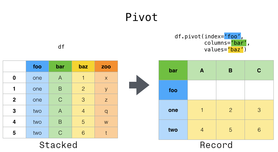
For the former, we need to “melt” the wide data, with multiple columns, into long data.
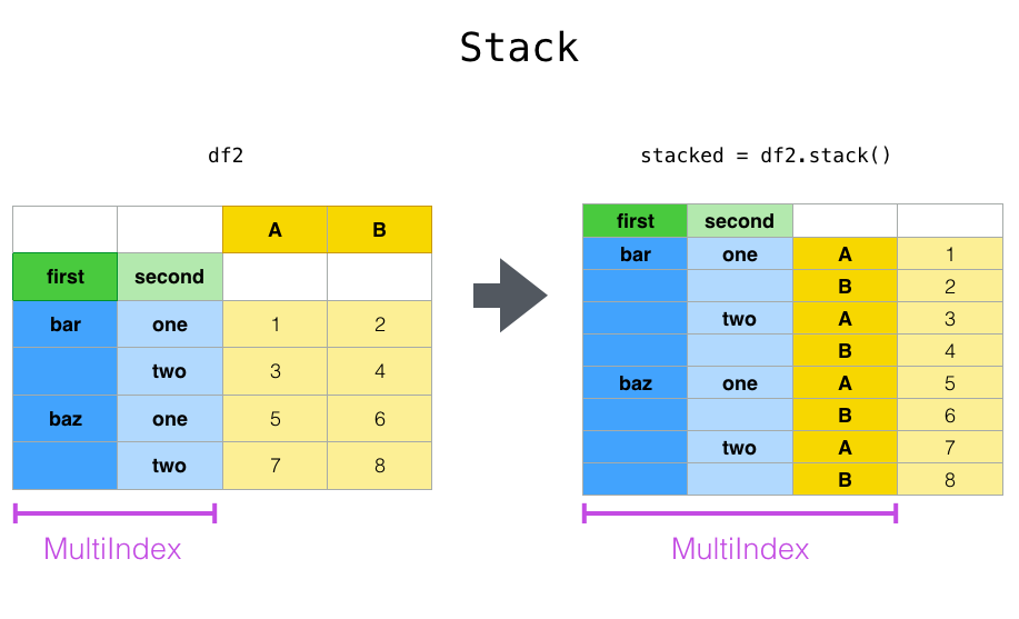
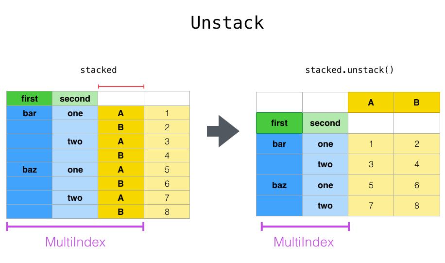
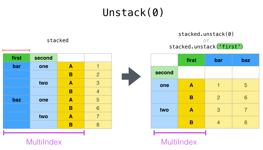
For the latter, we need to unstack or pivot the multiple rows into columns (ie go from long to wide.)
We’ll see both below.