Intro to Geo-Spatial Analysis

Introduction

In this chapter, you’ll learn the basics of geospatial analysis with code. This chapter is indebted to the excellent geographical shapefiles available to download from Natural Earth.

You should be aware when following this chapter that installing geographic analysis packages isn’t always the easiest and things can and do go wrong! (Some geospatial analysis courses recommend running everything in a Docker container.) If you’re not familiar with Docker and you’re installing everything locally, a strong recommendation is to use conda. There’s a brief guide on installing packages in the Chapter on Preliminaries.

There are two types of spatial data geographic information systems (GIS): vector and raster. Vector spatial data are made up of vertices and paths. These are represented computationally by points (zero-dimensional objects, if you like), lines (1D objects), and polygons (2D objects, aka an area). Vector data are analogous to vector image formats, like .eps and .pdf, they are smooth and well-defined regardless of the level of zoom you look at them (on a map). Raster data are composed of pixels, also known as grid cells. Each cell has a different value and the raster map is overlaid on a map. Raster data are better for continuous variables such as temperature or rainfall, while vector data are better suited to political boundaries and features like roads. In this book, we’ll only cover vector geospatial data analysis (if you need to work with rasters, check out rasterio).

Common file formats for vector data include Shapefile (.shp…), GeoJSON/JSON, KML and GeoPackage.

Coordinate Reference Systems

A Coordinate Reference System (CRS) associates numerical coordinates with a position on the surface of the Earth. Latitude and longitude are an example (and have units of degrees) but there are many CRSs. They are important because they define how your data will look on a map. Think about it like this: in the case of the usual charts you plot, you usually take it as given that you are working in a space that is 2D with an X- and Y-basis vector. But the most basic object in mapping is a sphere, which is fundamentally different to a 2D plane. This means you have to choose whether to show part of a globe or all of a 2D representation of a globe (a projection), which inevitably introduces distortions.

The type main classes of CRS are geographic or projection. A geographic CRS uses a 3D model of the Earth and ‘drapes’ the data over it.

A projected CRS has the geographic CRS plus a map projection that has co-ordinates on a 2D plane. It is well known that there is no distortion-free projection from a globe to a plane; you cannot preserve areas, shapes, distances, and angles simultaneously. Different map projections introduce different distortions, as lovingly shown in this xkcd cartoon.

One example of a map projection is the Mercator projection, which is a conformal mapping, i.e. a mapping that locally preserves angles, but not necessarily lengths. In fact, Mercator distorts areas, especially the further away an area is from the equator. Some projections are better for some purposes than others.

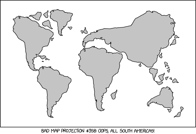
XKCD: Bad Map Projection: South America

Some analysis tools expect geospatial data to be in a projected CRS-this is true of the main package we’ll use, geopandas. This is usually not a problem for economic data; it’s rare that the curvature of the Earth becomes a factor (though distances might in some rare situations). Most spatial libraries expect that all of the data that are being combined be in the same CRS.

CRSs are usually referenced by an EPSG code. Two widely used CRSs are WGS84 (aka EPSG: 4326) which provides a good representation of most places on Earth and NAD83 (aka EPSG: 4269), which provides a good representation of the USA.

Why are we banging on about this? Because maps and geometry objects come in different CRS and it’s worth being aware of that so that you can ensure they are in the same format, and that you have the right CRS for your purposes.

Imports and packages

We’ll be using geopandas, the go-to package for vector spatial analysis in Python. The easiest way to install this package is using conda install geopandas; if you want to install it via pip then look at the install instructions.

Let’s import some of the packages we’ll be using:

import matplotlib.pyplot as plt
import pandas as pd
import os
import numpy as np
import geopandas as gpd
from pathlib import Path

# Set max rows displayed for readability
pd.set_option("display.max_rows", 6)
# Plot settings
plt.style.use(
    "https://github.com/aeturrell/coding-for-economists/raw/main/plot_style.txt"
)
# For this chapter, some bespoke settings:
plt.style.use(
    {
        "axes.autolimit_mode": "data",
        "patch.linewidth": 0.2,
        "figure.figsize": (10, 8),
        "figure.dpi": 125,
    }
)

Geopandas dataframes

Quite literally, GeoPandas is a combination of geo and pandas so the good news is that everything you know about using pandas dataframes can be re-used here for geospatial data. The geo part adds functionality for geo-spatial data.

Input and Output

So, first, we need some geo-spatial data to analyse. There are several different file formats for geo-spatial data, such as Shapefile (.shp), GeoJSON/JSON, KML, and GeoPackage.

We’ll use a Shapefile of the countries of the world from Natural Earth. It comes as a zip file; unzip it and one of the files ends in .shp, which is the one we load with geopandas.

Let’s load the data and look at the first few rows:

# To run this example, you will need to download the files at this url:
# https://github.com/aeturrell/coding-for-economists/tree/main/data/geo/world
# and save them in the path 'data/geo/world' (path relative to where you're running the code)
df = gpd.read_file(Path("data/geo/world/ne_50m_admin_0_countries.shp"))
df.head(3)

	featurecla	scalerank	LABELRANK	SOVEREIGNT	SOV_A3	ADM0_DIF	LEVEL	TYPE	ADMIN	ADM0_A3	...	NAME_KO	NAME_NL	NAME_PL	NAME_PT	NAME_RU	NAME_SV	NAME_TR	NAME_VI	NAME_ZH	geometry
0	Admin-0 country	1	3	Zimbabwe	ZWE	0	2	Sovereign country	Zimbabwe	ZWE	...	짐바브웨	Zimbabwe	Zimbabwe	Zimbábue	Зимбабве	Zimbabwe	Zimbabve	Zimbabwe	辛巴威	POLYGON ((31.28789 -22.40205, 31.19727 -22.344...
1	Admin-0 country	1	3	Zambia	ZMB	0	2	Sovereign country	Zambia	ZMB	...	잠비아	Zambia	Zambia	Zâmbia	Замбия	Zambia	Zambiya	Zambia	赞比亚	POLYGON ((30.39609 -15.64307, 30.25068 -15.643...
2	Admin-0 country	1	3	Yemen	YEM	0	2	Sovereign country	Yemen	YEM	...	예멘	Jemen	Jemen	Iémen	Йемен	Jemen	Yemen	Yemen	也门	MULTIPOLYGON (((53.08564 16.64839, 52.58145 16...

3 rows × 95 columns

There’s a lot of info here, but a lot of it is different labelling. The dataset has one country per row.

To save the data frame, use df.to_file("output_name.shp") for shapefiles. For other output formats use, for example, df.to_file("output_name.geojson", driver="GeoJSON").

Basics

Let’s see what we get when we call the humble plot function on the data we already read in!

df.plot(color="green");

I think it’s glorious just how easy this is to use.

Because geopandas builds on pandas, we can do all of the usual pandas-like operations such as filtering based on values. Here’s how to filter to an individual country (one with a recognisable shape!):

df[df["ADMIN"] == "Italy"].plot();

Note that it is the last column in the dataframe, the geometry column, that makes this sorcery possible.

Working with Coordinate Reference Systems

We can check what the CRS of this entire geopandas dataframe is:

df.crs

<Geographic 2D CRS: EPSG:4326>
Name: WGS 84
Axis Info [ellipsoidal]:
- Lat[north]: Geodetic latitude (degree)
- Lon[east]: Geodetic longitude (degree)
Area of Use:
- name: World.
- bounds: (-180.0, -90.0, 180.0, 90.0)
Datum: World Geodetic System 1984 ensemble
- Ellipsoid: WGS 84
- Prime Meridian: Greenwich

We can switch between CRS using the to_crs function. Let’s see the world map we plotted earlier using the WGS84 projection and also using some other projection, including the dreaded Meractor projection. Mercator looks completely ridiculous if we don’t drop Antarctica first, so let’s get shot of it for all the projections. (You can find a list of projections here.)

exclude_admins = ["Antarctica", "French Southern and Antarctic Lands"]
proj_names = ["WGS 84", "Mercator", "Winkel Tripel", "Quartic Authalic"]
crs_names = ["EPSG:4326", "EPSG:3395", "+proj=wintri", "+proj=qua_aut"]

world_no_antrtc = df[~df["ADMIN"].isin(exclude_admins)]

fig, axes = plt.subplots(
    nrows=2, ncols=2, figsize=(12, 6), dpi=150, sharex=False, sharey=False
)
for i, ax in enumerate(axes.flat):
    world_no_antrtc.to_crs(crs_names[i]).plot(ax=ax, color="#b2f3b2", linewidth=0.1)
    ax.set_title(proj_names[i])
    ax.axis("off")
plt.tight_layout()
plt.show();

Manipulating Space

Basics

Let’s look more closely at the objects that encode the shapes of the countries on our world map:

df.loc[df["ADMIN"] == "Italy", "geometry"]

137    MULTIPOLYGON (((7.02109 45.92578, 7.05576 45.9...
Name: geometry, dtype: geometry

The object is a multipolygon. Remember that we have points (0D), lines (1D), and polygons (aka areas, 2D) that we can embed in a projection. A line is at least 2 vertices that are connected; a polygon is the area contained within 3 or more vertices. Multipolygons are the union of two or more non-contiguous polygons: in this case, the Italian mainland, Sicily, and Sardinia.

The plot() function works just as happily if our basic objects are points rather than polygons though. In the below example, we’ll grab the centroid (the spatial midpoint) of each country as a point and plot them:

# We are going to round-trip the data through a flat projection that preserves
# area here, Equal Area Cylindrical ('+proj=cea'), and then convert back to a
# geographical CRS. This is to ensure the centroid results are correct across
# the globe. The key part is the `.centroid`
df["centroid"] = df.to_crs('+proj=cea').centroid.to_crs(df.crs)

fig, ax = plt.subplots()
ax.axis("off")
df.boundary.plot(ax=ax, lw=0.2, color="k")
df["centroid"].plot(ax=ax, color="red", markersize=15)
plt.show()

Let’s explore those basic building blocks a bit more. A point at position (1, 2) is defined as follows (shapely is used by geopandas):

from shapely.geometry import Point

point = Point(1, 2)
point

A point doesn’t have much other than a single position in 2D space. But lines have length, and polygons have area.

There are different kinds of lines but the simplest is the LineString() which can be constructed from a sequence of points.

from shapely.geometry import LineString

line = LineString(
    [Point(0.0, 1.0), Point(2.0, 2.0), Point(2.5, 5.0), Point(4, 5), Point(4, 0)]
)
print(f"Length of line is {line.length:.2f}")
line

Length of line is 11.78

We already saw Polygons in the shape of Italy. But here’s a much simpler one:

from shapely.geometry import Polygon

poly = Polygon([(0, 0), (1, 1), (1, 0)])
print(f"The area of the poly is {poly.area}")
poly

The area of the poly is 0.5

Spatial Operations

We’ve seen the basic building blocks of geometries: points, lines, and polygons. We’ve also seen how to retrieve some basic properties of these such as length, area, and centroid. In this section, we’ll see some slightly more advanced spatial operations that you can perform with geopandas.

Point-in-polygon

This does pretty much what you’d expect! It’s useful in practice because we might want to know if a particular place falls within one area or another. As a test, let’s see if the centroid for Germany actually falls within the Germany polygon.

df_row = df.loc[df["ADMIN"] == "Germany", :]
df_row["geometry"].iloc[0].contains(df_row["centroid"].iloc[0])

True

But be careful with this! Countries can have complex multi-polygon geometries for which a centroid is not guaranteed to be within any of the polygons. France is a great example as French Guiana is so far away that it pulls the centroid just out of the mainland:

fig, ax = plt.subplots()
df_row = df.loc[df["ADMIN"] == "France", :]
df_row["geometry"].plot(ax=ax)
df_row["centroid"].plot(ax=ax, color="red");

Buffers

Buffers are just an area drawn around a particular geometry, given a specific radius. They have a great practical use in computing catchment areas and so on. To create a buffer around the geometry you’re currently using, use the df.buffer(number) command to return a column with the buffered version of your geometry in. Be aware that the units of the CRS you’re using will determine the units of the buffer.

Spatial set operations

More complex spatial manipulation can be achieved through spatial set operations. The figure below shows some examples for polygons (but the same principles apply for lines and polygons too):

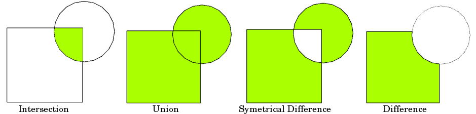
Different set operations with two polygons. Source: QGIS documentation.

In addition to these, there are ‘crosses’ (for two lines) and ‘touches’. You can find information about all of the set operations that are available here.

To demonstrate one of these, let’s see if we can pick out a few regions that are intersected by a river. We’ll try out the river Trent, which passes through England, and we’ll see which Local Authority Districts (LADs) it passes through. First, we load the UK data, which is from the ONS Open Geography Portal:

# To run this example, you will need to download the files at this url:
# https://github.com/aeturrell/coding-for-economists/tree/main/data/geo/uk_lad
# and save them in the path 'data/geo/uk_lad' (path relative to where you're running the code)
dfuk = gpd.read_file(
    Path("data/geo/uk_lad/Local_Authority_Districts__May_2020__UK_BUC.shp")
)
dfuk.plot(color="dimgrey");

Next we bring in data on major rivers and pass it through the same projection as our map of England is using:

# To run this example, you will need to download the files at this url:
# https://github.com/aeturrell/coding-for-economists/tree/main/data/geo/rivers
# and save them in the path 'data/geo/rivers' (path relative to where you're running the code)
river = gpd.read_file(Path("data/geo/rivers/rivers.shp"))
river = river.to_crs(dfuk.crs)
river.plot(color="mediumblue");

We can now combine these for a view on how these rivers goes through the UK. We will use buffer() to modify how easy it is to visualise the river by asking for everything within 1.5 km from the river.

fig, ax = plt.subplots(figsize=(15, 15))
ax.set_frame_on(False)
ax.set_xticks([])
ax.set_yticks([])
dfuk.plot(color="grey", ax=ax)
river.buffer(1.5e3).plot(ax=ax, color="lightblue");

Let’s turn our focus to one river: the Trent. We will ask which of the regions are intersected by that river and plot only those parts. We’ll also add some annotations for the names of the regions.

# Restrict river to just one
river_name = "Trent"
river = river[river["name"] == river_name]

# Find a subset of the regions that is intersected by the river by creating new True/False column
dfuk["river"] = dfuk["geometry"].apply(
    lambda x: river["geometry"].buffer(1e3).intersects(x)
)

# The rest of the code is just related to plotting:

# Create a cut of dfuk for convenience
df_th = dfuk[dfuk["river"]].copy()

# Get a representative point for each region to annotate
df_th["coords"] = (
    df_th["geometry"].representative_point().apply(lambda x: x.coords[:][0])
)

# Plotting bits
fig, ax = plt.subplots(figsize=(10, 10))
ax.set_frame_on(False)
ax.set_xticks([])
ax.set_yticks([])
df_th.plot(color="grey", ax=ax, edgecolor="0.6")
river.plot(color="lightblue", ax=ax)

# Add text annotation to the largest polygons
for idx, row in df_th.iterrows():
    if row["geometry"].area > np.quantile(df_th.area, q=0.4):
        ax.annotate(
            text=row["LAD20NM"],
            xy=row["coords"],
            horizontalalignment="center",
            weight="bold",
            fontsize=10,
            color="black",
        )
ax.set_title(
    f"Local Authority Districts that are intersected by the {river_name}",
    loc="left",
    fontsize=20,
)
plt.show()

Note that the way we set this up to use river_name as an input variable means we could oh so easily wrap everything up in a function that did this for other rivers. Oh go on then, let’s see how that works because it shows how scalable operations are once you do them in code:

def river_intersect_plot(river_name):
    """
    Given the name of a river, shows a plot of the LADs that it intersects.
    """
    river = gpd.read_file(os.path.join("data", "geo", "rivers", "rivers.shp"))
    river = river[river["name"] == river_name]
    river = river.to_crs(dfuk.crs)
    dfuk["river"] = dfuk["geometry"].apply(
        lambda x: river["geometry"].buffer(2e3).intersects(x)
    )
    df_th = dfuk[dfuk["river"]].copy()
    df_th["coords"] = (
        df_th["geometry"].representative_point().apply(lambda x: x.coords[:][0])
    )
    fig, ax = plt.subplots(figsize=(10, 10))
    ax.set_frame_on(False)
    ax.set_xticks([])
    ax.set_yticks([])
    df_th.plot(color="grey", ax=ax, edgecolor="0.6")
    river.plot(color="lightblue", ax=ax)
    for idx, row in df_th.iterrows():
        if row["geometry"].area > np.quantile(df_th.area, q=0.6):
            ax.annotate(
                text=row["LAD20NM"],
                xy=row["coords"],
                horizontalalignment="center",
                weight="bold",
                fontsize=10,
                color="black",
            )
    ax.set_title(
        f"Local Authority Districts that are intersected by the {river_name}",
        loc="left",
        fontsize=20,
    )
    plt.show()

With our function defined, we can do the whole thing for a completely different river:

river_intersect_plot("Thames")

Computing distances

Computing the distances between two points a and b (in the same CRS) is achieved using the a.distance(b) command.

As an example, let’s now find out how far it is between two regions of interest in our cut of regions around the Trent. We’ll pick the East Riding of Yorkshire and Stafford, and then plot them on the map in different colours. Because geopandas is so flexible, and there could be multiple geometries with the names ‘East Riding of Yorkshire’ and ‘Stafford’ we have to not only select the names we want but, in case there are multiple rows, specify which row. If you just want the first you can use iloc[0], which is what happens in the example below.

# Get the rows we're interested in out of the dataframe:
name_a = "East Riding of Yorkshire"
name_b = "Stafford"
# This selects the *all rows* that match these conditions, which is why we have to use .iloc[0] thereafter
# to make sure we're only passing a single row.
place_a = df_th.loc[df_th["LAD20NM"] == "East Riding of Yorkshire", :]
place_b = df_th.loc[df_th["LAD20NM"] == "Stafford", :]
# Compute the distance using representative points
dist_a_b = (
    place_a["geometry"]
    .representative_point()
    .iloc[0]
    .distance(place_b["geometry"].representative_point().iloc[0])
)

# Plot the map
fig, ax = plt.subplots(figsize=(10, 10))
ax.set_frame_on(False)
ax.set_xticks([])
ax.set_yticks([])
df_th.plot(color="grey", ax=ax, edgecolor="0.6")
river.plot(color="lightblue", ax=ax)
place_a.plot(ax=ax, color="red")
place_b.plot(ax=ax, color="green")
for i, place in enumerate([place_a, place_b]):
    ax.annotate(
        text=place["LAD20NM"].iloc[0],
        xy=place["coords"].iloc[0],
        horizontalalignment="center",
        weight="bold",
        fontsize=15,
        color="black",
    )
# Uncomment below to add a connecting line
## Create a line between two rep points in a and b
# connector = LineString([place_a['geometry'].representative_point().iloc[0],
#                        place_b['geometry'].representative_point().iloc[0]])
## Convert it to a geopandas dataframe for easy plotting
# gpd.GeoDataFrame([connector],columns=['line'], geometry='line').plot(ax=ax, linestyle='-.', color='black')
ax.set_title(
    f"Distance between {name_a} and {name_b} is {dist_a_b/1e3:1.0f} km.", loc="left"
)
plt.show()

Neighbours

It’s really useful to have a way to determine all of the adjacent geometries to a given geometry. The touches geospatial operation is the best for this but do be careful because the level of the detail in polygons varies for different maps and you may find that they sometimes overlap rather than simply touch. So, in the example of finding all of the neighbours for all of the local authority districts in the UK below, not only do we include those LADs that touch, we also include those that overlap.

# Empty list of lists
neighbours_all = [[] for _ in range(len(dfuk))]
# Iterate over rows
for index, row in dfuk.iterrows():
    # Find any touches of this row
    neighbours = dfuk.loc[dfuk["geometry"].touches(row["geometry"]), "LAD20NM"].tolist()
    # Find any overlaps of this row
    overlap = dfuk.loc[dfuk["geometry"].overlaps(row["geometry"]), "LAD20NM"].tolist()
    # Take the union of touches and overlaps
    neighbours = np.union1d(neighbours, overlap)
    # Store the result
    neighbours_all[index] = neighbours

# Put result back into geopandas dataframe (RHS is a list of lists of strings)
dfuk["neighbours"] = neighbours_all

Now we should have an extra column that tells us which regions are adjacent to which by name:

dfuk.head()

	OBJECTID	LAD20CD	LAD20NM	LAD20NMW	BNG_E	BNG_N	LONG	LAT	Shape__Are	Shape__Len	geometry	river	neighbours
0	1	E06000001	Hartlepool	None	447160	531474	-1.27018	54.6761	9.660727e+07	50737.909874	POLYGON ((448973.593 536745.277, 448986.025 53...	False	[County Durham, Stockton-on-Tees]
1	2	E06000002	Middlesbrough	None	451141	516887	-1.21099	54.5447	5.523093e+07	35500.289988	POLYGON ((451894.299 521145.303, 453997.697 51...	False	[Hambleton, Redcar and Cleveland, Stockton-on-...
2	3	E06000003	Redcar and Cleveland	None	464361	519597	-1.00608	54.5675	2.483255e+08	85085.268776	POLYGON ((478232.599 518788.828, 477689.303 51...	False	[Hambleton, Middlesbrough, Scarborough, Stockt...
3	4	E06000004	Stockton-on-Tees	None	444940	518183	-1.30664	54.5569	2.052160e+08	88846.876387	POLYGON ((452243.536 526335.188, 451711.300 52...	False	[County Durham, Darlington, Hambleton, Hartlep...
4	5	E06000005	Darlington	None	428029	515648	-1.56835	54.5353	1.988128e+08	91926.839545	POLYGON ((436388.002 522354.197, 437351.702 52...	False	[County Durham, Hambleton, Richmondshire, Stoc...

Let’s plot an example to be sure we’ve done it all right!

name_of_region = "High Peak"
# Set colors now for ease in plotting
dfuk["color"] = "#b2df8a"
dfuk.loc[dfuk["LAD20NM"] == name_of_region, "color"] = "#33a02c"
# Get representative points to use for text annotation. Note that we want xy coords, hence the fussy use of .apply
dfuk["coords"] = dfuk["geometry"].representative_point().apply(lambda x: x.coords[:][0])
# Get a list of the neighbours--again, this comes out as a dataframe row so we need to call iloc[0] to get first entry
names_neighbours = list(
    dfuk.loc[dfuk["LAD20NM"] == name_of_region, "neighbours"].iloc[0]
)
# Cut to only those areas of interest
df_cut = dfuk.loc[dfuk["LAD20NM"].isin(names_neighbours + [name_of_region])]

fig, ax = plt.subplots(figsize=(10, 10))
df_cut.plot(ax=ax, color=df_cut["color"], edgecolor="k")
ax.set_frame_on(False)
ax.set_xticks([])
ax.set_yticks([])
# Add annotation
for idx, row in df_cut.iterrows():
    ax.annotate(
        text=row["LAD20NM"],
        xy=row["coords"],
        horizontalalignment="center",
        weight="bold",
        fontsize=15,
        color="black",
    )
plt.show()

Hooray! It looks like it worked. And notice how the only variable we need to change to get a different map is name_of_region, so this could easily be wrapped up in a function to re-use again.

For an exercise, why don’t you see if you can figure out what’s so special about Powys and the Isle of Wight.

Aggregation and Dissolve

Dissolve

A useful common map operation is to aggregate by spatial region: i.e. to eliminate some of the granularity of a map by combining smaller regions into larger regions. This is called a ‘dissolve’ because it dissolves the boundaries between regions to form larger ones.

To demonstrate it, let’s take the many UK local authority districts and dissolve() them into the UK countries. We can do this using the LAD20CD column because the code used for it always begins with a letter that represents the country: E for England, W for Wales, N for Northern Ireland, and S for Scotland. So to do the dissolve, we first create a new column just like we would do for a groupby() in a regular pandas dataframe. But instead of using groupby(), we dissolve() by the new column. This will give us a new map that is made up of only 4 polygons.

dfuk["country"] = dfuk["LAD20CD"].apply(lambda x: str(x)[0])
dfuk.iloc[:, [1, 2, -1]].head()

	LAD20CD	LAD20NM	country
0	E06000001	Hartlepool	E
1	E06000002	Middlesbrough	E
2	E06000003	Redcar and Cleveland	E
3	E06000004	Stockton-on-Tees	E
4	E06000005	Darlington	E

country_uk = dfuk.dissolve(by="country")
country_uk.plot(edgecolor="k");

The default way that columns other than the geometry are combined is by taking the first row of each kind, but dissolve accepts and agg_func= argument that you can also pass last, min, max, sum, mean, and median.

Aggregation

Because geopandas builds on pandas, all the usual operations (i.e. groupby()) that you might do on a pandas dataframe also work for non-geometry columns.

Merging data

Attribute Joins

In an attribute join, a GeoSeries or GeoDataFrame is combined with a regular pandas Series or DataFrame based on a common variable. This is analogous to normal merging or joining in pandas.

Spatial Joins

Spatial joins are more complex because we take two different sets of geometries and say how to combine them. The key to this is i) ensuring that the datasets have the same CRS and ii) using sjoin() to perform the spatial join. We’ll show how to do a spatial join that is an inner intersection using op=intersects.

We’ll take some data on, and a map of, the world, which has per country geometries in plus columns for, eg, gdp per capita, and we’ll merge it with a dataframe with the names and positions of cities in. Our intersects spatial join will combine each city (a lat/lon point) with the shapes of countries and determine which city goes in which country (even if it’s on the boundary).

This is just one example of a spatial join: the other possible arguments to op are within and contains.

# To run this example, you will need to download the files at this url:
# https://github.com/aeturrell/coding-for-economists/tree/main/data/geo/detailed_world
# and save them in the path 'data/geo/detailed_world' (path relative to where you're running the code)
# Grab a world map that has extra data in
world = gpd.read_file(Path("data/geo/detailed_world/ne_110m_admin_0_countries.shp"))
# drop columns we're less interested in
cols_to_keep = ['featurecla', 'scalerank', 'LABELRANK', 'SOVEREIGNT', 'SOV_A3', 'ADM0_DIF', 'LEVEL', 'TYPE', 'ADMIN', 'POP_EST', "geometry"]
world = world.loc[:, cols_to_keep]
world.head()

	featurecla	scalerank	LABELRANK	SOVEREIGNT	SOV_A3	ADM0_DIF	LEVEL	TYPE	ADMIN	POP_EST	geometry
0	Admin-0 country	1	6	Fiji	FJI	0	2	Sovereign country	Fiji	889953.0	MULTIPOLYGON (((180.00000 -16.06713, 180.00000...
1	Admin-0 country	1	3	United Republic of Tanzania	TZA	0	2	Sovereign country	United Republic of Tanzania	58005463.0	POLYGON ((33.90371 -0.95000, 34.07262 -1.05982...
2	Admin-0 country	1	7	Western Sahara	SAH	0	2	Indeterminate	Western Sahara	603253.0	POLYGON ((-8.66559 27.65643, -8.66512 27.58948...
3	Admin-0 country	1	2	Canada	CAN	0	2	Sovereign country	Canada	37589262.0	MULTIPOLYGON (((-122.84000 49.00000, -122.9742...
4	Admin-0 country	1	2	United States of America	US1	1	2	Country	United States of America	328239523.0	MULTIPOLYGON (((-122.84000 49.00000, -120.0000...

# To run this example, you will need to download the files at this url:
# https://github.com/aeturrell/coding-for-economists/tree/main/data/geo/cities
# and save them in the path 'data/geo/cities' (path relative to where you're running the code)
cities = gpd.read_file(Path("data/geo/cities/ne_110m_populated_places.shp"))
cities = cities.to_crs(world.crs)
cols_to_keep_cities = ["FEATURECLA", 'NAME', 'NAMEPAR', 'NAMEALT', 'NAMEASCII', "geometry", "LATITUDE", "LONGITUDE"]
cities = cities.loc[:, cols_to_keep_cities]
cities.head()

	FEATURECLA	NAME	NAMEPAR	NAMEALT	NAMEASCII	geometry	LATITUDE	LONGITUDE
0	Admin-0 capital	Vatican City	None	None	Vatican City	POINT (12.45339 41.90328)	41.903282	12.453387
1	Admin-0 capital	San Marino	None	None	San Marino	POINT (12.44177 43.93610)	43.936096	12.441770
2	Admin-0 capital	Vaduz	None	None	Vaduz	POINT (9.51667 47.13372)	47.133724	9.516670
3	Admin-0 capital alt	Lobamba	None	None	Lobamba	POINT (31.20000 -26.46667)	-26.466668	31.199997
4	Admin-0 capital	Luxembourg	None	None	Luxembourg	POINT (6.13000 49.61166)	49.611660	6.130003

cities_with_country = gpd.sjoin(cities, world, how="inner", predicate="intersects")
cities_with_country.head()

	FEATURECLA	NAME	NAMEPAR	NAMEALT	NAMEASCII	geometry	LATITUDE	LONGITUDE	index_right	featurecla	scalerank	LABELRANK	SOVEREIGNT	SOV_A3	ADM0_DIF	LEVEL	TYPE	ADMIN	POP_EST
0	Admin-0 capital	Vatican City	None	None	Vatican City	POINT (12.45339 41.90328)	41.903282	12.453387	141	Admin-0 country	1	2	Italy	ITA	0	2	Sovereign country	Italy	60297396.0
1	Admin-0 capital	San Marino	None	None	San Marino	POINT (12.44177 43.93610)	43.936096	12.441770	141	Admin-0 country	1	2	Italy	ITA	0	2	Sovereign country	Italy	60297396.0
226	Admin-0 capital	Rome	None	None	Rome	POINT (12.48131 41.89790)	41.897902	12.481313	141	Admin-0 country	1	2	Italy	ITA	0	2	Sovereign country	Italy	60297396.0
2	Admin-0 capital	Vaduz	None	None	Vaduz	POINT (9.51667 47.13372)	47.133724	9.516670	114	Admin-0 country	1	4	Austria	AUT	0	2	Sovereign country	Austria	8877067.0
212	Admin-0 capital	Vienna	Wien	None	Vienna	POINT (16.36469 48.20196)	48.201961	16.364693	114	Admin-0 country	1	4	Austria	AUT	0	2	Sovereign country	Austria	8877067.0

Now we have our cities, and their points, merged into a dataset that also gives the continent and other data that was originally only in our world dataframe.

Geocoding

Geocoding is the process of taking an address or the name of a place and retrieving its position in a geographic co-ordinate system. There are many entities you might want to do this for, such as cities, landmarks, geographic features like rivers, and postal code. Reverse geocoding takes a latitude and longitude and works backwards to work out the name of the object that’s there.

Geocoding as a service is offered by several providers, including Geocodio, Google’s geocode API service, Bing, OpenStreetMap, and more. Some of these charge, especially for volume.

There are two parts of geocoding: one is the interface that you use to issue the command (the front-end, the bit you see), and another is that does the actual geocoding (the back-end, an API you don’t see). The back-end bit is what you sometimes have to pay for as a service if you’re geocoding at scale.

We’ll look at a geocoding package that comes in two different forms: Geopy, which is a Python package that provides a front end for a large number of geocoding APIs, including OpenStreetMap, Bing, Google, ArcGIS, and more. You may also want to explore the geocoder Python package as an alternative.

Geopy stand-alone

Below is an example of using Geopy as a stand-alone package. We’ll use the OpenStreetMap API to do the geocoding, which is called Nominatim. It’s important to note that this API has some fair usage conditions including a maximum of 1 request per second, that you provide an informative ‘user agent’ parameter, and that you clearly display attribution (thank you OpenStreetMap!). For bulk geocoding, you may need to pay a fee to a provider.

Let’s see an example retrieving the full address of a landmark:

# If you don't have it, install geopy using 'pip install geopy'
from geopy.geocoders import Nominatim

# Create a geolocator using Open Street Map (aka Nominatim)
# Use your own user agent identifier here
geolocator = Nominatim(user_agent="codeforecon")

# Pass an address to retrieve full location information:
location = geolocator.geocode("Bank of England")

location.address

'Bank of England, 8AH, Threadneedle Street, Cornhill, City of London, Greater London, England, EC2R 8AH, United Kingdom'

The location parameter also contains a latitude and longitude, which is useful for further geospatial operations:

(location.latitude, location.longitude)

(51.51413225, -0.08892476721255456)

And here’s an example of using the same API to do a reverse geocode from a given lat/lon:

# We can also reverse geocode from a lat and lon:
scnd_location = geolocator.reverse("51.529969, -0.127688")

scnd_location.address

'British Library, 96, Euston Road, Somers Town, London Borough of Camden, London, Greater London, England, NW1 2DB, United Kingdom'

Geopy built-in to geopandas

If you don’t want to break out into a separate package, you need not! geopandas has its own interface with geopy. We’ll use it to get the boroughs of ..

boros_df = gpd.GeoDataFrame(
    {"boro_name": ["Staten Island", "Queens", "Brooklyn", "Manhattan", "Bronx"]},
    index=range(5),
)
boros_df.head()

	boro_name
0	Staten Island
1	Queens
2	Brooklyn
3	Manhattan
4	Bronx

Next we carry out the geocoding step using gpd.tools.geocode() and pass an entire column of values that we would like to get POINT geometries and address for:

boros_df[["geometry", "address"]] = gpd.tools.geocode(boros_df.boro_name, provider="photon")
boros_df

/Users/aet/mambaforge/envs/codeforecon/lib/python3.10/site-packages/pandas/core/frame.py:4123: FutureWarning: You are adding a column named 'geometry' to a GeoDataFrame constructed without an active geometry column. Currently, this automatically sets the active geometry column to 'geometry' but in the future that will no longer happen. Instead, either provide geometry to the GeoDataFrame constructor (GeoDataFrame(... geometry=GeoSeries()) or use `set_geometry('geometry')` to explicitly set the active geometry column.
  self[k1] = value[k2]

	boro_name	geometry	address
0	Staten Island	POINT (-74.14960 40.58346)	Staten Island, New York, New York, United States
1	Queens	POINT (-73.82831 40.71351)	Queens, New York, New York, United States
2	Brooklyn	POINT (-73.94972 40.65260)	Brooklyn, New York, New York, United States
3	Manhattan	POINT (-73.95989 40.78962)	Manhattan, New York, New York, United States
4	Bronx	POINT (-73.87859 40.84665)	The Bronx, New York, New York, United States

OpenStreetMap and Osmnx

OpenStreetMap (OSM) is a crowd-sourced project that aims to create a free map of the world containing information about streets, buildings, landmarks, landuse, and more. Its users regularly update the information it holds. Think Wikipedia but for a world map. It excels at highly detailed and freely available renderings of streets.

Osmnx is a package that can retrieve, construct, analyze, and visualize street networks from OpenStreetMap [Boeing, 2017]. It also does some geocoding on the fly. Let’s see it in action and feed in the address we obtained in the geocoding example from earlier; using the graph_from_point() method will give us the network of streets around a location.

import osmnx as ox

# Fetch OSM street network from the location
graph = ox.graph_from_point(
    (location.latitude, location.longitude), dist=1.3e3, network_type="all"
)

The returned object is of type multidigraph, or more precisely networkx.classes.multidigraph.MultiDiGraph. This is an object defined in the networkx package, and you can find out more about its properties here but what’s important is that, at least here, the network’s nodes are where streets meet and its edges are streets.

Rather than plot this as nodes and edges, we can make a much nicer plot of the grid of streets using the below snippet:

fig, ax = ox.plot_graph(
    graph, bgcolor="white", node_size=0, edge_color="grey", show=False, close=False
)
plt.show()

The channel with few streets is the river Thames.

We can also use osmnx to work out the shortest path between nodes. Let’s see a practical example: going from Bank, north of the river Thames, to Borough Market (great for lunch), south of the river. First, we need the lat and long of Borough Market.

lunch_loc = geolocator.geocode("Borough Market")
lunch_loc.address

'Borough Market, Cathedral Street, Bankside, The Borough, London Borough of Southwark, London, Greater London, England, SE1 9DE, United Kingdom'

Now we find the nearest node to the given locations, and ask osmnx to work out a route.

orig = ox.nearest_nodes(graph, Y=location.latitude, X=location.longitude)
dest = ox.nearest_nodes(graph, Y=lunch_loc.latitude, X=lunch_loc.longitude)
route = ox.shortest_path(graph, orig, dest)

fig, ax = ox.plot_graph_route(
    graph,
    route,
    route_linewidth=4,
    node_size=0,
    bgcolor="white",
    show=False,
    close=False,
    route_color="r",
)
plt.show()

Okay, you’re in Borough Market but you need to decide where exactly to get your lunch from. OpenStreetMap includes information on many kinds of nearby amenities, including bar, cafe, and pub. We can retrieve this information and put it straight into a geopandas dataframe using the geometries_from_place() function.

restaurants = ox.features_from_place(
    "Borough Market", tags={"amenity": "restaurant"},
)

def plot_osm_geoms(osm_df, skip_names=5):
    osm_df["coords"] = (
        osm_df["geometry"].representative_point().apply(lambda x: x.coords[:][0])
    )
    fig, ax = ox.plot_graph(
        graph, bgcolor="white", node_size=0, edge_color="grey", show=False, close=False
    )
    osm_df.plot(ax=ax, color="blue", alpha=0.6)
    for idx, row in osm_df[::skip_names].iterrows():
        ax.annotate(
            text=row["name"],
            xy=row["coords"],
            xytext=(-30, -40),
            textcoords="offset points",
            horizontalalignment="center",
            weight="bold",
            fontsize=10,
            color="black",
            arrowprops=dict(
                arrowstyle="->",
                color="k",
                connectionstyle="arc3,rad=0.3",
                lw=1.5,
            ),
        )
    plt.show()


plot_osm_geoms(restaurants)

amenity is just one type of geometry that can be retrieved too: others are building, landuse, and leisure. You can find a list of them here. For example, here are the (many) churches in the City of London:

churches = ox.features_from_place(
    "City of London", tags={"building": "church"}
)
churches = churches.dropna(subset=["name"])

plot_osm_geoms(churches, skip_names=7)

Review

If you know:

• ✅ what a coordinate reference system (crs) is;

• ✅ how to open and use geospatial data using geopandas;

• ✅ how to create quick plots of maps;

• ✅ what points, lines, and polygons are in a geospatial context;

• ✅ how to perform set operations on points, lines, and polygons;

• ✅ how to compute distances, nearest neighbours, and other geospatial properties;

• ✅ how to aggregate, merge, and dissolve geospatial data; and

• ✅ how to use geocoding to retrieve geospatial data

then you have a good grasp of the basics of geospatial analysis!