import matplotlib.pyplot as plt
import numpy as np
import pandas as pd

# Set seed for random numbers
seed_for_prng = 78557
prng = np.random.default_rng(
    seed_for_prng
) # prng=probabilistic random number generatorData Transformation
Introduction
The previous chapter showed how to access different parts of a dataframe and create new rows or columns. In this chapter, you’ll learn how to do more interesting transformations of data including aggregations and groupbys.
This chapter is hugely indebted to the fantastic Python Data Science Handbook by Jake Vanderplas. Remember, if you get stuck with pandas, there is brilliant documentation and a fantastic set of introductory tutorials on the pandas website. These notes are heavily indebted to those introductory tutorials.
Prerequisites
This chapter uses the pandas and numpy packages. If you’re running this code, you may need to install these packages, which you can do using either conda install packagename or pip install packagename on your computer’s command line. If you’re running this page in Google Colab, you can install new packages by running !pip install packagename in a new code cell but you will need to restart the Colab notebook for the change to take effect. There’s a brief guide on installing packages in the Chapter on Preliminaries. Remember, you only need to install them once!
Aggregation
Aggregation means taking some data and applying a statistical operation that aggregates the information into a smaller number of statistics. Because aggregations take many numbers and produce, typically, fewer numbers, they involve a function of some kind. While you can always write your own aggregation functions, pandas has some common ones built in—and these can be applied to rows or columns as we’ll see.
The pandas built-in aggregation functions include:
| Aggregation | Description |
|---|---|
count() |
Number of items |
first(), last() |
First and last item |
mean(), median() |
Mean and median |
min(), max() |
Minimum and maximum |
std(), var() |
Standard deviation and variance |
mad() |
Mean absolute deviation |
prod() |
Product of all items |
sum() |
Sum of all items |
value_counts() |
Counts of unique values |
these can applied to all entries in a dataframe, or optionally to rows or columns using axis=0 or axis=1 (or "rows" or "columns") respectively. Here are a couple of examples using the sum() function (note that we aggregate over rows leaving only columns):
df = pd.DataFrame(np.random.randint(0, 5, (3, 5)), columns=list("ABCDE"))
df| A | B | C | D | E | |
|---|---|---|---|---|---|
| 0 | 2 | 0 | 1 | 2 | 3 |
| 1 | 2 | 1 | 4 | 2 | 1 |
| 2 | 2 | 3 | 1 | 2 | 4 |
df.sum(axis=0)A 6
B 4
C 6
D 6
E 8
dtype: int64df.sum(axis="rows")A 6
B 4
C 6
D 6
E 8
dtype: int64
TipExercise
Find the mean values of each column (eg leaving only column headers so aggregating over rows using axis=0) and the mean values of each row (eg leaving only row headers and therefore aggregating over columns using axis=1)
If you want to create custom aggregations, you can of course do that too using the apply() method from Working with Data.
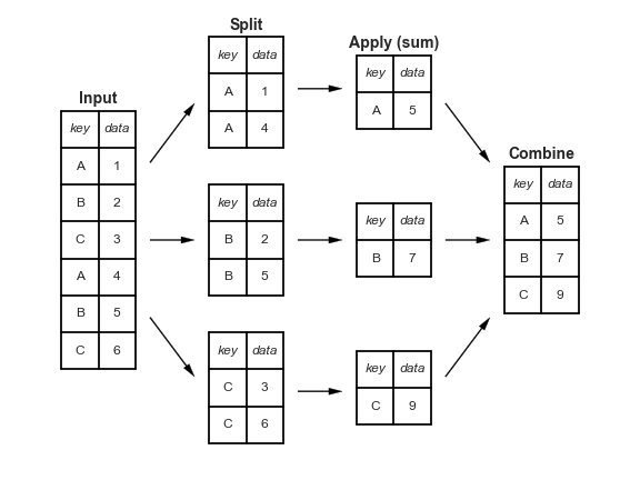
Groupby and then aggregate (aka split, apply, combine)
Splitting a dataset, applying a function, and combining the results are three key operations that we’ll want to use together again and again. Splitting means differentiating between rows or columns of data based on some conditions, for instance different categories or different values. Applying means applying a function, for example finding the mean or sum. Combine means putting the results of these operations back into the dataframe, or into a variable. The figure gives an example
A very common way of doing this is using the groupby() operation to group rows according to come common property. The classic use-case would be to find the mean by a particular characteristic, perhaps the mean height by gender. Note that the ‘combine’ part at the end doesn’t always have to result in a new dataframe; it could create new columns in an existing dataframe (but the new column is the result of a groupby operation, eg subtracting a group mean).
Let’s first see a really simple example of splitting a dataset into groups and finding the mean across those groups using the penguins dataset. We’ll group the data by island and look at the means.
penguins = pd.read_csv(
    "https://raw.githubusercontent.com/mwaskom/seaborn-data/master/penguins.csv"
)
penguins["sex"] = penguins["sex"].str.title()
penguins.head()| species | island | bill_length_mm | bill_depth_mm | flipper_length_mm | body_mass_g | sex | |
|---|---|---|---|---|---|---|---|
| 0 | Adelie | Torgersen | 39.1 | 18.7 | 181.0 | 3750.0 | Male |
| 1 | Adelie | Torgersen | 39.5 | 17.4 | 186.0 | 3800.0 | Female |
| 2 | Adelie | Torgersen | 40.3 | 18.0 | 195.0 | 3250.0 | Female |
| 3 | Adelie | Torgersen | NaN | NaN | NaN | NaN | NaN |
| 4 | Adelie | Torgersen | 36.7 | 19.3 | 193.0 | 3450.0 | Female |
penguins.groupby("island").mean(numeric_only=True)| bill_length_mm | bill_depth_mm | flipper_length_mm | body_mass_g | |
|---|---|---|---|---|
| island | ||||
| Biscoe | 45.257485 | 15.874850 | 209.706587 | 4716.017964 |
| Dream | 44.167742 | 18.344355 | 193.072581 | 3712.903226 |
| Torgersen | 38.950980 | 18.429412 | 191.196078 | 3706.372549 |
The aggregations from the previous part all work on grouped data. An example is df['body_mass_g'].groupby('island').median() for the median body mass by island.
TipExercise
Using a groupby, find the standard deviation of different penguin species’ body measurements. (Hint: standard deviation has its own aggregation/combine function given by std())
Multiple Functions using agg()
You can also pass multiple functions via the agg() method (short for aggregation). Here we pass two numpy functions (these two functions have built-in equivalents std() and mean() so this is just for illustrative purposes):
penguins.groupby("species")[penguins.select_dtypes("number").columns].agg(
    ["mean", "std"]
)| bill_length_mm | bill_depth_mm | flipper_length_mm | body_mass_g | |||||
|---|---|---|---|---|---|---|---|---|
| mean | std | mean | std | mean | std | mean | std | |
| species | ||||||||
| Adelie | 38.791391 | 2.663405 | 18.346358 | 1.216650 | 189.953642 | 6.539457 | 3700.662252 | 458.566126 |
| Chinstrap | 48.833824 | 3.339256 | 18.420588 | 1.135395 | 195.823529 | 7.131894 | 3733.088235 | 384.335081 |
| Gentoo | 47.504878 | 3.081857 | 14.982114 | 0.981220 | 217.186992 | 6.484976 | 5076.016260 | 504.116237 |
TipExercise
Trying the obvious keywords, find the max and min of all columns grouping by island.
Multiple aggregations can also be performed at once on the entire dataframe by using a dictionary to map columns into functions. You can also group by as many variables as you like by passing the groupby method a list of variables. Here’s an example that combines both of these features:
penguins.groupby(["species", "island"]).agg(
    {"body_mass_g": "sum", "bill_length_mm": "mean"}
)| body_mass_g | bill_length_mm | ||
|---|---|---|---|
| species | island | ||
| Adelie | Biscoe | 163225.0 | 38.975000 |
| Dream | 206550.0 | 38.501786 | |
| Torgersen | 189025.0 | 38.950980 | |
| Chinstrap | Dream | 253850.0 | 48.833824 |
| Gentoo | Biscoe | 624350.0 | 47.504878 |
TipExercise
Using a two-column groupby() on species and island and an agg, use a dictionary to find the min of bill_depth_mm and the max of flipper_length_mm
Sometimes, inheriting the column names using agg() is problematic. There’s a slightly fussy syntax to help with that. It uses tuples, which are values within parenthesis (eg () that have the pattern (column name, function name). To the left of the tuple, you can specify a new name for the resulting column. Here’s an example:
penguins.groupby(["species", "island"]).agg(
    count_bill=("bill_length_mm", "count"),
    mean_bill=("bill_length_mm", "mean"),
    std_flipper=("flipper_length_mm", "std"),
)| count_bill | mean_bill | std_flipper | ||
|---|---|---|---|---|
| species | island | |||
| Adelie | Biscoe | 44 | 38.975000 | 6.729247 |
| Dream | 56 | 38.501786 | 6.585083 | |
| Torgersen | 51 | 38.950980 | 6.232238 | |
| Chinstrap | Dream | 68 | 48.833824 | 7.131894 |
| Gentoo | Biscoe | 123 | 47.504878 | 6.484976 |
TipExercise
Using a two-column groupby() on species and island and a named agg(), create a new column called mean_flipper that gives the mean of flipper_length_mm.
Filter
Filtering does exactly what it sounds like, but it can make use of group-by commands. In the example below, all but one species is filtered out.
In the example below, filter() passes a grouped version of the dataframe into the filter_func() we’ve defined (imagine that a dataframe is passed for each group). Because the passed variable is a dataframe, and variable x is defined in the function, the x within filter_func() body behaves like our dataframe–including having the same columns.
def filter_func(x):
    return x["bill_length_mm"].mean() > 48


penguins.groupby("species").filter(filter_func).head()| species | island | bill_length_mm | bill_depth_mm | flipper_length_mm | body_mass_g | sex | |
|---|---|---|---|---|---|---|---|
| 152 | Chinstrap | Dream | 46.5 | 17.9 | 192.0 | 3500.0 | Female |
| 153 | Chinstrap | Dream | 50.0 | 19.5 | 196.0 | 3900.0 | Male |
| 154 | Chinstrap | Dream | 51.3 | 19.2 | 193.0 | 3650.0 | Male |
| 155 | Chinstrap | Dream | 45.4 | 18.7 | 188.0 | 3525.0 | Female |
| 156 | Chinstrap | Dream | 52.7 | 19.8 | 197.0 | 3725.0 | Male |
Transform
Transforms return a transformed version of the data that has the same shape as the input (typically with an intermediate groupby). Think of it as split-apply-combine but without the ‘combine’ part! This is useful when creating new columns that depend on some grouped data, for instance creating group-wise means. Below is a synthetic example using the datetime group to subtract a yearly mean. We’ll create our synthetic example using some data, a datetime index, and some groups:
index = pd.date_range("1/1/2000", periods=10, freq="QE")
data = np.random.randint(0, 10, (10, 2))
df = pd.DataFrame(data, index=index, columns=["values1", "values2"])
df["type"] = np.random.choice(["group" + str(i) for i in range(3)], 10)
df| values1 | values2 | type | |
|---|---|---|---|
| 2000-03-31 | 4 | 6 | group1 |
| 2000-06-30 | 9 | 5 | group2 |
| 2000-09-30 | 2 | 3 | group0 |
| 2000-12-31 | 3 | 9 | group1 |
| 2001-03-31 | 0 | 9 | group0 |
| 2001-06-30 | 8 | 8 | group1 |
| 2001-09-30 | 8 | 9 | group1 |
| 2001-12-31 | 3 | 2 | group1 |
| 2002-03-31 | 3 | 2 | group2 |
| 2002-06-30 | 9 | 7 | group1 |
Now we take the yearly means by type. pd.Grouper(freq='A') is an instruction to take the Annual mean using the given datetime index. You can group on as many coloumns and/or index properties as you like: this example groups by a property of the datetime index and on the type column, but performs the computation on the values1 column.
df["v1_demean_yr_and_type"] = df.groupby([pd.Grouper(freq="A"), "type"])[
    "values1"
].transform(lambda x: x - x.mean())
df
/var/folders/x6/ffnr59f116l96_y0q0bjfz7c0000gn/T/ipykernel_46304/2763383649.py:1: FutureWarning: 'A' is deprecated and will be removed in a future version, please use 'YE' instead.
df["v1_demean_yr_and_type"] = df.groupby([pd.Grouper(freq="A"), "type"])[| values1 | values2 | type | v1_demean_yr_and_type | |
|---|---|---|---|---|
| 2000-03-31 | 4 | 6 | group1 | 0.500000 |
| 2000-06-30 | 9 | 5 | group2 | 0.000000 |
| 2000-09-30 | 2 | 3 | group0 | 0.000000 |
| 2000-12-31 | 3 | 9 | group1 | -0.500000 |
| 2001-03-31 | 0 | 9 | group0 | 0.000000 |
| 2001-06-30 | 8 | 8 | group1 | 1.666667 |
| 2001-09-30 | 8 | 9 | group1 | 1.666667 |
| 2001-12-31 | 3 | 2 | group1 | -3.333333 |
| 2002-03-31 | 3 | 2 | group2 | 0.000000 |
| 2002-06-30 | 9 | 7 | group1 | 0.000000 |
TipExercise
Create a new column that gives values2 normalised (minus the mean and divided by standard deviation) by type.
Assign
Assign is a method that allows you to return a new object with all the original columns in addition to new ones. Existing columns that are re-assigned will be overwritten. This is really useful when you want to perform a bunch of operations together in a concise way and keep the original columns. To show it in action, let’s generate some data:
For instance, to demean the ‘values1’ column by year-type and to recompute the ‘val1_times_val2’ column using the newly demeaned ‘values1’ column:
df.assign(
    values1=(
        df.groupby([pd.Grouper(freq="A"), "type"])["values1"].transform(
            lambda x: x - x.mean()
        )
    ),
    val1_times_val2=lambda x: x["values1"] * x["values2"],
)
/var/folders/x6/ffnr59f116l96_y0q0bjfz7c0000gn/T/ipykernel_46304/1721473601.py:3: FutureWarning: 'A' is deprecated and will be removed in a future version, please use 'YE' instead.
df.groupby([pd.Grouper(freq="A"), "type"])["values1"].transform(| values1 | values2 | type | v1_demean_yr_and_type | val1_times_val2 | |
|---|---|---|---|---|---|
| 2000-03-31 | 0.500000 | 6 | group1 | 0.500000 | 3.000000 |
| 2000-06-30 | 0.000000 | 5 | group2 | 0.000000 | 0.000000 |
| 2000-09-30 | 0.000000 | 3 | group0 | 0.000000 | 0.000000 |
| 2000-12-31 | -0.500000 | 9 | group1 | -0.500000 | -4.500000 |
| 2001-03-31 | 0.000000 | 9 | group0 | 0.000000 | 0.000000 |
| 2001-06-30 | 1.666667 | 8 | group1 | 1.666667 | 13.333333 |
| 2001-09-30 | 1.666667 | 9 | group1 | 1.666667 | 15.000000 |
| 2001-12-31 | -3.333333 | 2 | group1 | -3.333333 | -6.666667 |
| 2002-03-31 | 0.000000 | 2 | group2 | 0.000000 | 0.000000 |
| 2002-06-30 | 0.000000 | 7 | group1 | 0.000000 | 0.000000 |
TipExercise
Re-write the transform function from the transform exercise (creating a normalised column transformed by type) as an assign statement with a new column name transformed_by_type.
agg(), transform(), and apply(): when to use each with a groupby
With all of the different options available, it can be confusing to know when to use the different functions available for performing groupby operations, namely: .agg(), .transform(), and .apply(). Here are the key points to remember:
- Use
.agg()when using a groupby, but you want your groups to become the new index - Use
.transform()when using a groupby, but you want to retain your original index - Use
.apply()when using a groupby, but you want to perform operations that will leave neither the original index nor an index of groups
Let’s see an example of all three on a series (pd.Series()) to really highlight the differences. First, let’s create the series:
len_s = 1000
s = pd.Series(
    index=pd.date_range("2000-01-01", periods=len_s, name="date", freq="D"),
    data=prng.integers(-10, 10, size=len_s),
)
s.head()
date
2000-01-01 7
2000-01-02 -4
2000-01-03 -9
2000-01-04 7
2000-01-05 0
Freq: D, dtype: int64Okay, now we can try these three operations out successively with some example functions. We’ll use skew for the first two, .agg() and .transform, in order to highlight that the only difference between these is in the index that is returned. For .agg(), using lambda x: x.skew() would return the same as .agg() in this case so we’ll opt for a more interesting example: only using values greater than zero and then taking their cumulative sum. Note that what is returned in this third case is an object with a multi-index: the first index tracks the groupby groups while the second tracks the original rows that survived the filtering to values greater than zero.
print("\n`.agg` following `.groupby`: groups provide index")
print(s.groupby(s.index.to_period("M")).agg("skew").head())
print("\n`.transform` following `.groupby`: retain original index")
print(s.groupby(s.index.to_period("M")).transform("skew").head())
print("\n`.apply` following `.groupby`: index entries can be new")
print(s.groupby(s.index.to_period("M")).apply(lambda x: x[x > 0].cumsum()).head())
`.agg` following `.groupby`: groups provide index
date
2000-01    0.110284
2000-02    0.223399
2000-03    0.003857
2000-04    0.122812
2000-05   -0.039962
Freq: M, dtype: float64

`.transform` following `.groupby`: retain original index
date
2000-01-01    0.110284
2000-01-02    0.110284
2000-01-03    0.110284
2000-01-04    0.110284
2000-01-05    0.110284
Freq: D, dtype: float64

`.apply` following `.groupby`: index entries can be new
date     date
2000-01  2000-01-01     7
         2000-01-04    14
         2000-01-06    23
         2000-01-07    29
         2000-01-12    38
dtype: int64
Reshaping Data
The main options for reshaping data are pivot(), melt(), stack(), unstack(), pivot_table(), get_dummies(), cross_tab(), and explode(). We’ll look at some of these here.
Pivoting data from tidy to, err, untidy
In a previous chapter, we said you should use tidy data–one row per observation, one column per variable–whenever you can. But there are times when you will want to take your lovingly prepared tidy data and pivot it into a wider format. pivot() and pivot_table() help you to do that.
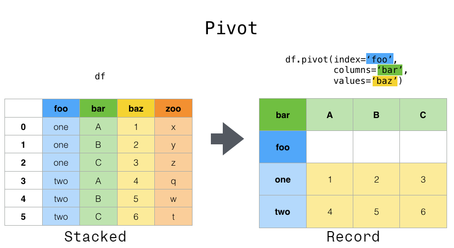
This can be especially useful for time series data, where operations like shift() or diff() are typically applied assuming that an entry in one row follows (in time) from the one above. Here’s an example:
data = {
    "value": np.random.randn(20),
    "variable": ["A"] * 10 + ["B"] * 10,
    "category": prng.choice(["type1", "type2", "type3", "type4"], 20),
    "date": (
        list(pd.date_range("1/1/2000", periods=10, freq="M"))
        + list(pd.date_range("1/1/2000", periods=10, freq="M"))
    ),
}
df = pd.DataFrame(data, columns=["date", "variable", "category", "value"])
df.sample(5)
/var/folders/x6/ffnr59f116l96_y0q0bjfz7c0000gn/T/ipykernel_46304/12375816.py:6: FutureWarning: 'M' is deprecated and will be removed in a future version, please use 'ME' instead.
list(pd.date_range("1/1/2000", periods=10, freq="M"))
/var/folders/x6/ffnr59f116l96_y0q0bjfz7c0000gn/T/ipykernel_46304/12375816.py:7: FutureWarning: 'M' is deprecated and will be removed in a future version, please use 'ME' instead.
+ list(pd.date_range("1/1/2000", periods=10, freq="M"))| date | variable | category | value | |
|---|---|---|---|---|
| 0 | 2000-01-31 | A | type1 | 0.950327 |
| 10 | 2000-01-31 | B | type1 | 0.512804 |
| 13 | 2000-04-30 | B | type3 | -0.581118 |
| 12 | 2000-03-31 | B | type1 | 0.547337 |
| 2 | 2000-03-31 | A | type2 | -0.610155 |
If we just run shift() on this, it’s going to shift variable B’s and A’s together even though these overlap in time. So we pivot to a wider format (and then we can shift safely).
df.pivot(index="date", columns="variable", values="value").shift(1)| variable | A | B |
|---|---|---|
| date | ||
| 2000-01-31 | NaN | NaN |
| 2000-02-29 | 0.950327 | 0.512804 |
| 2000-03-31 | -0.734731 | -0.259099 |
| 2000-04-30 | -0.610155 | 0.547337 |
| 2000-05-31 | 0.250122 | -0.581118 |
| 2000-06-30 | -0.815883 | -0.690586 |
| 2000-07-31 | 1.996651 | 0.035080 |
| 2000-08-31 | 0.483854 | 0.622108 |
| 2000-09-30 | -1.999759 | 1.674825 |
| 2000-10-31 | -0.121439 | 0.863201 |
To go back to the original structure, albeit without the category columns, apply .unstack().reset_index().
TipExercise
Perform a pivot that applies to both the variable and category columns. (Hint: remember that you will need to pass multiple objects via a list.)
Melt
melt() can help you go from untidy to tidy data (from wide data to long data), and is a really good one to remember. Of course, if you’re a normal human, you’ll have to look back at the documentation most times you use this!
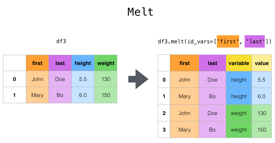
Here’s an example of it in action:
df = pd.DataFrame(
    {
        "first": ["John", "Mary"],
        "last": ["Doe", "Bo"],
        "job": ["Nurse", "Economist"],
        "height": [5.5, 6.0],
        "weight": [130, 150],
    }
)
print("\n Unmelted: ")
print(df)
print("\n Melted: ")
df.melt(id_vars=["first", "last"], var_name="quantity", value_vars=["height", "weight"])
 Unmelted:
  first last        job  height  weight
0  John  Doe      Nurse     5.5     130
1  Mary   Bo  Economist     6.0     150

Melted: | first | last | quantity | value | |
|---|---|---|---|---|
| 0 | John | Doe | height | 5.5 |
| 1 | Mary | Bo | height | 6.0 |
| 2 | John | Doe | weight | 130.0 |
| 3 | Mary | Bo | weight | 150.0 |
TipExercise
Perform a melt that uses job as the id instead of first and last.
If you don’t wan the headscratching of melt, there’s also wide_to_long(), which is really useful for typical data cleaning cases where you have data like this:
df = pd.DataFrame(
    {
        "A1970": {0: "a", 1: "b", 2: "c"},
        "A1980": {0: "d", 1: "e", 2: "f"},
        "B1970": {0: 2.5, 1: 1.2, 2: 0.7},
        "B1980": {0: 3.2, 1: 1.3, 2: 0.1},
        "X": dict(zip(range(3), np.random.randn(3))),
        "id": dict(zip(range(3), range(3))),
    }
)
df| A1970 | A1980 | B1970 | B1980 | X | id | |
|---|---|---|---|---|---|---|
| 0 | a | d | 2.5 | 3.2 | 0.941307 | 0 |
| 1 | b | e | 1.2 | 1.3 | 2.659910 | 1 |
| 2 | c | f | 0.7 | 0.1 | 0.175392 | 2 |
i.e. data where there are different variables and time periods across the columns. Wide to long is going to let us give info on what the stubnames are (‘A’, ‘B’), the name of the variable that’s always across columns (here, a year), any values (X here), and an id column.
pd.wide_to_long(df, stubnames=["A", "B"], i="id", j="year")| X | A | B | ||
|---|---|---|---|---|
| id | year | |||
| 0 | 1970 | 0.941307 | a | 2.5 |
| 1 | 1970 | 2.659910 | b | 1.2 |
| 2 | 1970 | 0.175392 | c | 0.7 |
| 0 | 1980 | 0.941307 | d | 3.2 |
| 1 | 1980 | 2.659910 | e | 1.3 |
| 2 | 1980 | 0.175392 | f | 0.1 |
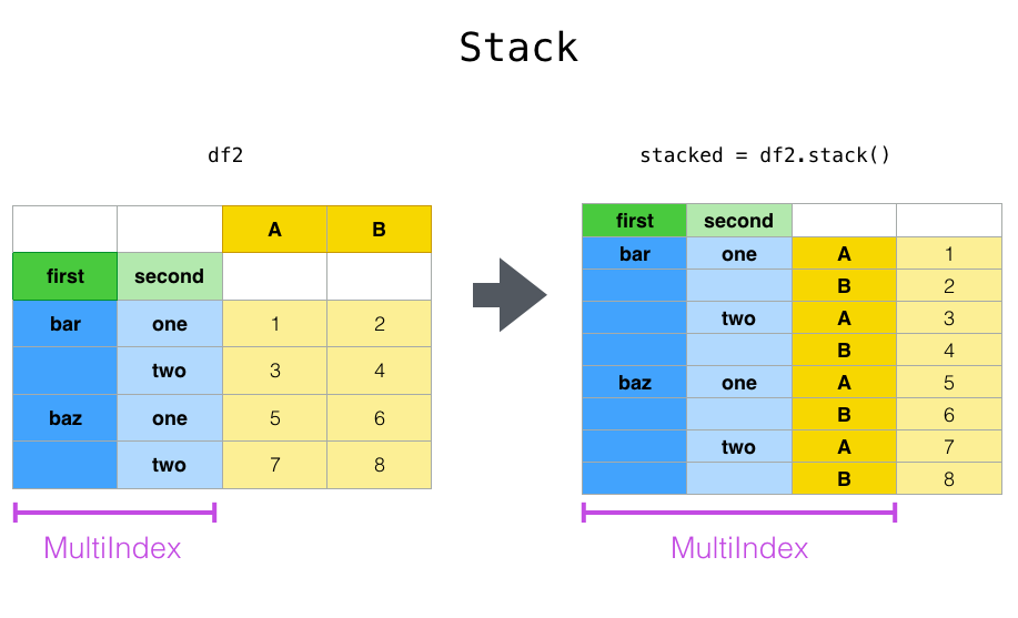
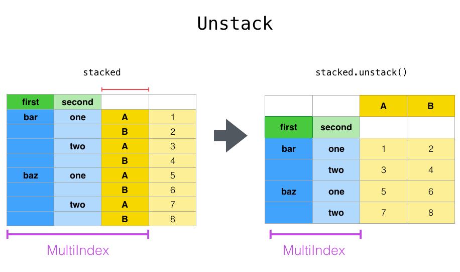
Stack and unstack
Stack, stack() is a shortcut for taking a single type of wide data variable from columns and turning it into a long form dataset, but with an extra index.
Unstack, unstack() unsurprisingly does the same operation, but in reverse.
Let’s define a multi-index dataframe to demonstrate this:
tuples = list(
    zip(
        *[
            ["bar", "bar", "baz", "baz", "foo", "foo", "qux", "qux"],
            ["one", "two", "one", "two", "one", "two", "one", "two"],
        ]
    )
)
index = pd.MultiIndex.from_tuples(tuples, names=["first", "second"])
df = pd.DataFrame(np.random.randn(8, 2), index=index, columns=["A", "B"])
df| A | B | ||
|---|---|---|---|
| first | second | ||
| bar | one | -1.629067 | 1.195897 |
| two | -0.119983 | 0.949348 | |
| baz | one | 0.073124 | -1.034615 |
| two | -0.978438 | -0.641276 | |
| foo | one | -0.878422 | 0.681782 |
| two | 0.076719 | -0.291882 | |
| qux | one | -1.297756 | -0.850906 |
| two | 1.519175 | 0.144894 |
Let’s stack this to create a tidy dataset:
df = df.stack()
df
first second
bar one A -1.629067
B 1.195897
two A -0.119983
B 0.949348
baz one A 0.073124
B -1.034615
two A -0.978438
B -0.641276
foo one A -0.878422
B 0.681782
two A 0.076719
B -0.291882
qux one A -1.297756
B -0.850906
two A 1.519175
B 0.144894
dtype: float64This has automatically created a multi-layered index but that can be reverted to a numbered index using df.reset_index()
Now let’s see unstack but, instead of unstacking the ‘A’, ‘B’ variables we began with, let’s unstack the ‘first’ column by passing level=0 (the default is to unstack the innermost index). This diagram shows what’s going on:
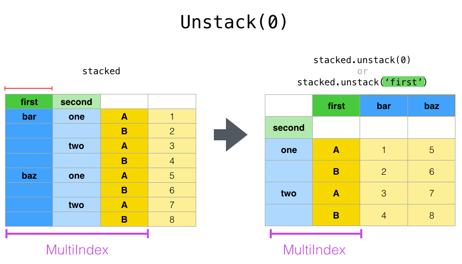
And here’s the code:
df.unstack(level=0)| first | bar | baz | foo | qux | |
|---|---|---|---|---|---|
| second | |||||
| one | A | -1.629067 | 0.073124 | -0.878422 | -1.297756 |
| B | 1.195897 | -1.034615 | 0.681782 | -0.850906 | |
| two | A | -0.119983 | -0.978438 | 0.076719 | 1.519175 |
| B | 0.949348 | -0.641276 | -0.291882 | 0.144894 |
TipExercise
What happens if you unstack to level=1 instead? What about applying unstack() twice?
Get dummies
This is a really useful reshape command for when you want (explicit) dummies in your dataframe. When running simple regressions, you can achieve the same effect by declaring the column only be included as a fixed effect, but there are some machine learning packages where converting to dummies may be easier.
Here’s an example:
df = pd.DataFrame(
    {"group_var": ["group1", "group2", "group3"], "B": ["c", "c", "b"], "C": [1, 2, 3]}
)
print(df)

pd.get_dummies(df, columns=["group_var"])
group_var B C
0 group1 c 1
1 group2 c 2
2 group3 b 3| B | C | group_var_group1 | group_var_group2 | group_var_group3 | |
|---|---|---|---|---|---|
| 0 | c | 1 | True | False | False |
| 1 | c | 2 | False | True | False |
| 2 | b | 3 | False | False | True |
A quick look at time series and rolling windows
The support for time series and the datetime type is excellent in pandas and in Python in general; you can find more about this in Introduction to Time and more on how to use time series with pandas in Time Series.
It is very easy to manipulate datetimes with pandas. The relevant part of the documentation has more info; here we’ll just see a couple of the most important bits. First, let’s create some synthetic data to work with:
def recursive_ts(n, x=0.05, beta=0.6, alpha=0.2):
    shock = np.random.normal(loc=0, scale=0.6)
    if n == 0:
        return beta * x + alpha + shock
    else:
        return beta * recursive_ts(n - 1, x=x) + alpha + shock


t_series = np.cumsum([recursive_ts(n) for n in range(12)])
index = pd.date_range("1/1/2000", periods=12, freq="M")
df = pd.DataFrame(t_series, index=index, columns=["values"])
df.loc["2000-08-31", "values"] = np.nan
df
/var/folders/x6/ffnr59f116l96_y0q0bjfz7c0000gn/T/ipykernel_46304/2804880687.py:10: FutureWarning: 'M' is deprecated and will be removed in a future version, please use 'ME' instead.
index = pd.date_range("1/1/2000", periods=12, freq="M")| values | |
|---|---|
| 2000-01-31 | -0.556188 |
| 2000-02-29 | -0.985137 |
| 2000-03-31 | -0.339044 |
| 2000-04-30 | -0.399989 |
| 2000-05-31 | 0.010603 |
| 2000-06-30 | 0.961386 |
| 2000-07-31 | -0.399649 |
| 2000-08-31 | NaN |
| 2000-09-30 | 1.128552 |
| 2000-10-31 | 0.814264 |
| 2000-11-30 | 1.399946 |
| 2000-12-31 | 2.015916 |
Now let’s imagine that there are a number of issues with this time series. First, it’s been recorded wrong: it actually refers to the start of the next month, not the end of the previous as recorded; second, there’s a missing number we want to interpolate; third, we want to take the difference of it to get to something stationary; fourth, we’d like to add a lagged column. We can do all of those things!
# Change freq to next month start
df.index += pd.tseries.offsets.DateOffset(days=1)

# impute the value that is NaN (Not a Number) above
df["values"] = df["values"].interpolate(method="time")

# Take first differences
df["diff_values"] = df["values"].diff(1)

# Create a lag of the first differences
df["lag_diff_values"] = df["diff_values"].shift(1)
df| values | diff_values | lag_diff_values | |
|---|---|---|---|
| 2000-02-01 | -0.556188 | NaN | NaN |
| 2000-03-01 | -0.985137 | -0.428948 | NaN |
| 2000-04-01 | -0.339044 | 0.646093 | -0.428948 |
| 2000-05-01 | -0.399989 | -0.060945 | 0.646093 |
| 2000-06-01 | 0.010603 | 0.410592 | -0.060945 |
| 2000-07-01 | 0.961386 | 0.950783 | 0.410592 |
| 2000-08-01 | -0.399649 | -1.361036 | 0.950783 |
| 2000-09-01 | 0.376977 | 0.776627 | -1.361036 |
| 2000-10-01 | 1.128552 | 0.751574 | 0.776627 |
| 2000-11-01 | 0.814264 | -0.314288 | 0.751574 |
| 2000-12-01 | 1.399946 | 0.585683 | -0.314288 |
| 2001-01-01 | 2.015916 | 0.615970 | 0.585683 |
Having performed these operations, can you see why the "lag_diff_value" column has two entries that are NaN?
TipExercise
Add a lead that is 3 months ahead of values.
Two other useful time series functions to be aware of are resample() and rolling(). resample() can upsample or downsample time series. Downsampling is by aggregation, eg df['values].resample('Q').mean() to downsample to quarterly (‘Q’) frequency by taking the mean within each quarter. Upsampling involves a choice about how to fill in the missing values; examples of options are bfill() (backfill) and ffill() (forwards fill).
Rolling is for taking rolling aggregations, as you’d expect; for example, the 3-month rolling mean of our first difference time series:
df["diff_values"].rolling(3).mean()2000-02-01 NaN
2000-03-01 NaN
2000-04-01 NaN
2000-05-01 0.052066
2000-06-01 0.331913
2000-07-01 0.433477
2000-08-01 0.000113
2000-09-01 0.122125
2000-10-01 0.055722
2000-11-01 0.404638
2000-12-01 0.340990
2001-01-01 0.295788
Name: diff_values, dtype: float64Rolling Groupby
Often there are times when you’d like to compute the rolling mean at the group level, for example for each state. Here’s a typical example of this, and how to compute the grouped rolling mean. This example comes from the excellent calmcode website.
First, let’s pick up some data that we might want to apply this to and ensure the "date" column has the datetime datatype:
df = pd.read_csv("https://calmcode.io/static/data/birthdays.csv")
df["date"] = pd.to_datetime(df["date"])
df = df.set_index("date")
df.head()| state | year | month | day | wday | births | |
|---|---|---|---|---|---|---|
| date | ||||||
| 1969-01-01 | AK | 1969 | 1 | 1 | Wed | 14 |
| 1969-01-01 | AL | 1969 | 1 | 1 | Wed | 174 |
| 1969-01-01 | AR | 1969 | 1 | 1 | Wed | 78 |
| 1969-01-01 | AZ | 1969 | 1 | 1 | Wed | 84 |
| 1969-01-01 | CA | 1969 | 1 | 1 | Wed | 824 |
Note that we added a datetime index above; this is because .rolling() likes to have a datetime index to work on.
What we’ll do now is proceed in two steps:
- Group the data with
.groupby(). Each grouped set will have an index attached and we’re getting a grouped-series object because we’re only selecting the births column. - Use
.transform()to perform an operation only within groups.
df["rolling_births"] = df.groupby("state")["births"].transform(
    lambda x: x.rolling("30D", min_periods=1).mean()
)
df.head()| state | year | month | day | wday | births | rolling_births | |
|---|---|---|---|---|---|---|---|
| date | |||||||
| 1969-01-01 | AK | 1969 | 1 | 1 | Wed | 14 | 14.0 |
| 1969-01-01 | AL | 1969 | 1 | 1 | Wed | 174 | 174.0 |
| 1969-01-01 | AR | 1969 | 1 | 1 | Wed | 78 | 78.0 |
| 1969-01-01 | AZ | 1969 | 1 | 1 | Wed | 84 | 84.0 |
| 1969-01-01 | CA | 1969 | 1 | 1 | Wed | 824 | 824.0 |
To check that the result is something sensible, you can always sort the dataframe by date and group. Here, that lets us check that the rolling births are indeed following the births column in the way that we expect.
df = df.sort_index().sort_values(by="state")
df.head()| state | year | month | day | wday | births | rolling_births | |
|---|---|---|---|---|---|---|---|
| date | |||||||
| 1969-01-01 | AK | 1969 | 1 | 1 | Wed | 14 | 14.000000 |
| 1985-02-20 | AK | 1985 | 2 | 20 | Wed | 45 | 34.100000 |
| 1981-03-15 | AK | 1981 | 3 | 15 | Sun | 20 | 26.633333 |
| 1976-10-20 | AK | 1976 | 10 | 20 | Wed | 16 | 22.000000 |
| 1972-11-12 | AK | 1972 | 11 | 12 | Sun | 22 | 18.466667 |
For a more in-depth look at combining groups with rolling aggregations, take a look at the tutorial on calmcode.
There is much more on time series with pandas in the Chapter on Time Series.
Method Chaining
Warning
Method Chaining is a more advanced topic; feel free to skip it.
Sometimes, rather than splitting operations out into multiple lines, it can be more concise and clear to chain methods together. A typical time you might do this is when reading in a dataset and perfoming all of the initial cleaning. Tom Augsperger has a great tutorial on this, which I’ve reproduced parts of here. For more info on the pipe function used below, check out these short video tutorials.
To chain methods together, both the input and output must be a pandas dataframe. Many functions already do input and output these, for example the df.rename(columns={'old_col': 'new_col'}) takes in df and outputs a dataframe with one column name changed.
But occasionally, we’ll want to use a function that we’ve defined (rather than an already existing one). For that, we need the pipe method; it ‘pipes’ the result of one operation to the next operation. When objects are being passed through multiple functions, this can be much clearer. Compare, for example,
f(g(h(df), g_arg=a), f_arg=b)that is, dataframe df is being passed to function h, and the results of that are being passed to a function g that needs a key word argument g_arg, and the results of that are being passed to a function f that needs keyword argument f_arg. The nested structure is barely readable. Compare this with
(df.pipe(h)
   .pipe(g, g_arg=a)
   .pipe(f, f_arg=b)
)
Let’s see a method chain in action on a real dataset so you get a feel for it. We’ll use 1,000 rows of flight data from BTS (a popular online dataset for demos of data cleaning!). (For further info on method chaining in Python, see these videos–but be aware they assume advanced knowledge of the language.)
df = pd.read_csv(
    "https://github.com/aeturrell/coding-for-economists/raw/main/data/flights1kBTS.csv",
    index_col=0,
)
df.head()| FL_DATE | OP_UNIQUE_CARRIER | TAIL_NUM | ORIGIN | ORIGIN_CITY_NAME | DEST | DEST_CITY_NAME | DEP_TIME | ARR_TIME | ARR_DELAY | CANCELLATION_CODE | AIR_TIME | DISTANCE | Unnamed: 13 | |
|---|---|---|---|---|---|---|---|---|---|---|---|---|---|---|
| 403296 | 2020-01-20 | G4 | 231NV | SFB | Sanford, FL | AVL | Asheville, NC | 2011.0 | 2137.0 | 6.0 | NaN | 64.0 | 465.0 | NaN |
| 126199 | 2020-01-06 | MQ | N687JS | ORD | Chicago, IL | MSN | Madison, WI | 1837.0 | 1927.0 | -16.0 | NaN | 26.0 | 109.0 | NaN |
| 417268 | 2020-01-20 | YV | N516LR | IAD | Washington, DC | DTW | Detroit, MI | 1738.0 | 1915.0 | 14.0 | NaN | 60.0 | 383.0 | NaN |
| 67589 | 2020-01-04 | OO | N804SK | SAV | Savannah, GA | DTW | Detroit, MI | 653.0 | 844.0 | -26.0 | NaN | 91.0 | 705.0 | NaN |
| 102760 | 2020-01-05 | WN | N789SW | SAN | San Diego, CA | TUS | Tucson, AZ | 732.0 | 941.0 | -19.0 | NaN | 53.0 | 368.0 | NaN |
We’ll try and do a number of operations in one go: putting column titles in lower case, discarding useless columns, creating precise departure and arrival times, turning some of the variables into categoricals, creating a demeaned delay time, and creating a new categorical column for distances according to quantiles that will be called ‘near’, ‘less near’, ‘far’, and ‘furthest’. Some of these operations require a separate function, so we first define those. When we do the cleaning, we’ll pipe our dataframe to those functions (optionally passing any arguments).
def extract_city_name(df):
    """
    Chicago, IL -> Chicago for origin_city_name and dest_city_name
    """
    cols = ["origin_city_name", "dest_city_name"]
    city = df[cols].apply(lambda x: x.str.extract("(.*), \w{2}", expand=False))
    df = df.copy()
    df[["origin_city_name", "dest_city_name"]] = city
    return df


def time_to_datetime(df, columns):
    """
    Combine all time items into datetimes.

    2014-01-01,0914 -> 2014-01-01 09:14:00
    """
    df = df.copy()

    def converter(col):
        timepart = (
            col.astype(str)
            .str.replace("\.0$", "", regex=True)  # NaNs force float dtype
            .str.pad(4, fillchar="0")
        )
        return pd.to_datetime(
            df["fl_date"]
            + " "
            + timepart.str.slice(0, 2)
            + ":"
            + timepart.str.slice(2, 4),
            errors="coerce",
        )

    df[columns] = df[columns].apply(converter)
    return df


df = (
    df.drop([x for x in df.columns if "Unnamed" in x], axis=1)
    .rename(columns=str.lower)
    .pipe(extract_city_name)
    .pipe(time_to_datetime, ["dep_time", "arr_time"])
    .assign(
        fl_date=lambda x: pd.to_datetime(x["fl_date"]),
        dest=lambda x: pd.Categorical(x["dest"]),
        origin=lambda x: pd.Categorical(x["origin"]),
        tail_num=lambda x: pd.Categorical(x["tail_num"]),
        arr_delay=lambda x: pd.to_numeric(x["arr_delay"]),
        op_unique_carrier=lambda x: pd.Categorical(x["op_unique_carrier"]),
        arr_delay_demean=lambda x: x["arr_delay"] - x["arr_delay"].mean(),
        distance_group=lambda x: (
            pd.qcut(x["distance"], 4, labels=["near", "less near", "far", "furthest"])
        ),
    )
)
df.head()| fl_date | op_unique_carrier | tail_num | origin | origin_city_name | dest | dest_city_name | dep_time | arr_time | arr_delay | cancellation_code | air_time | distance | arr_delay_demean | distance_group | |
|---|---|---|---|---|---|---|---|---|---|---|---|---|---|---|---|
| 403296 | 2020-01-20 | G4 | 231NV | SFB | Sanford | AVL | Asheville | 2020-01-20 20:11:00 | 2020-01-20 21:37:00 | 6.0 | NaN | 64.0 | 465.0 | 8.544995 | less near |
| 126199 | 2020-01-06 | MQ | N687JS | ORD | Chicago | MSN | Madison | 2020-01-06 18:37:00 | 2020-01-06 19:27:00 | -16.0 | NaN | 26.0 | 109.0 | -13.455005 | near |
| 417268 | 2020-01-20 | YV | N516LR | IAD | Washington | DTW | Detroit | 2020-01-20 17:38:00 | 2020-01-20 19:15:00 | 14.0 | NaN | 60.0 | 383.0 | 16.544995 | less near |
| 67589 | 2020-01-04 | OO | N804SK | SAV | Savannah | DTW | Detroit | 2020-01-04 06:53:00 | 2020-01-04 08:44:00 | -26.0 | NaN | 91.0 | 705.0 | -23.455005 | far |
| 102760 | 2020-01-05 | WN | N789SW | SAN | San Diego | TUS | Tucson | 2020-01-05 07:32:00 | 2020-01-05 09:41:00 | -19.0 | NaN | 53.0 | 368.0 | -16.455005 | less near |