Reproducible Analysis

Introduction

This chapter will tell you about reproducible analysis and what are sometimes called “reproducible analytical pipelines”, also known as RAPs. This chapter has benefitted from the “Quality Assurance of Code for Analysis and Research” book produced by the Best Practice and Impact division of the Office for National Statistics and “The Turing Way”, a guide to reproducibility produced by the Alan Turing Institute.

Reproducibility can mean a lot of things to a lot of different people in a lot of different contexts. Here, we’re going to think about the reproducibility of analysis performed by code. That excludes external validity and although it might include robust coding practices, it doesn’t include robustness checks.

It does include Reproducible Analytical Pipelines (RAPs), which are automated analytical processes. At their best, RAPs use elements of software engineering best practice to ensure that analysis is reproducible.

There are different levels and aspects of reproducibile analysis with code, which we will step through in the rest of this chapter, but they form a hierarchy:

• modular code

• sensible, isolated project structure using relative filepaths

• an unmodified version of the raw data is retained; outputs can be regenerated

• operations should form a reproducible analytical pipeline

• the reproducible analytical pipeline can be automatically executed (eg using Make or a ‘main’ script)

• code language is reproducible (eg Python=3.8.12 in pyproject.toml file)

• code language packages are reproducible (eg pandas=1.3.3 in pyproject.toml file)

• code language packages’ dependencies are reproducible (eg pandas depends on numpy=1.21 as specified in poetry.lock file)

• operating system is reproducible (as specified in a Docker file or by using repo2docker)

A lot of the value to be had in reproducible code can be achieved by just the first five. Nailing all but the last one is a high standard and probably the right spot in the trade-off between effort and reproducibility for a lot of projects. If you get this far, you’re doing a really great job. Doing all of these is the gold standard.

Reproducibility isn’t just about ensuring your results reproduce, though that’s obviously the main reason to do it. It’s also about saving you time and effort. This image, from biological psychiatry researcher Daniel Quintana’s talk Five things about open and reproducible science that every early career researcher should know, sums it up nicely:

Using Modular Code

(You may have already met this idea before as the DRY, or “don’t repeat yourself”, concept).

How you structure your code can itself aid reproducibility. Let’s imagine you have a situation where you want to perform two similar analytical tasks in which the only thing that changes are the inputs and outputs. Let’s say, for example, that you want to perform a particular set of operations, perhaps the following:

find the mean from the second entry in a list onwards, add 1, divide by the number of entries in the reduced length list and then print the answer as a score

Here’s one example of that:

import numpy as np

list1 = [3, 4, 5, 6, 7, 8]
score1 = (np.mean(list1[1:]) + 1) / 5
print(f"The score is {score1:.2f}")

The score is 1.40

But now we have imagine we have a second set of variables we’d like to run the same logic on. Naively, you might copy and paste the same code again but replace the list with the new one, like this:

list2 = [16, 12, 88, 1, 9, 7, 32, 5]
score2 = (np.mean(list2[1:]) + 1) / 5
print(f"The score is {score2:.2f}")

The score is 4.60

The problem with this is that we repeated the code even though we wanted to perform the same operation, which is not very efficient.

We also expect score1 and score2 to be using the same operations, but we can’t be sure now because the code is different. And indeed, in this case, the copy and paste philosophy has gone wrong. Did you spot the mistake? Instead of dividing by the number of entries in the reduced length list, our copy and paste job saw us dividing by the number of entries in the first case (creating score1).

What we should have done is create modular code, where the same logic is not repeated but re-used. In this case, that’s best done with a function like follows:

def compute_score(list_input):
    """find the mean from the second entry in a list onwards,
    add 1, divide by the number of entries in the reduced
    length list and then print the answer as a score.

    Args:
        list_input (list[float]): A list of numbers
    Returns:
        score (float): A computed score
    """
    reduced_list = list_input[1:]
    score = (np.mean(reduced_list) + 1) / len(reduced_list)
    print(f"The score is {score:.2f}")


# Just to show it works:
compute_score(list1)
compute_score(list2)

The score is 1.40
The score is 3.29

We can now be sure that we get exactly the same set of operations applied each time because we put the logic into one function that is called for both lists. And, to avoid any copy and paste errors, we switched from hard-coding the divisor to making it part of the logic of the function (by dividing by len(reduced_list)).

By putting our logic in a function, we’ve also made what we are trying to do clearer to the reader—and remember, coders, that reader is most likely to be you in a few months time.

Functions help with reproducibile analytical pipelines because you can be sure that even if your inputs change slightly, the same logic or set of operations will be run.

Of course, functions do not have to be in the same script (the same .py file) as the one you are currently writing your code in. Python allows you to import functions from other scripts.

A classic example would be if you had a project that was structured like this:

📁 project
│──main.py
│──utilities.py
│──figures.py
│──README.md

where ‘project’ is a folder, and the files within it are three Python scripts and a markdown document. Your utilities script might have a really useful function in it that you’d like to use in main.py and figures.py too. You can do this! It’s possible to do from ‘within’ your other scripts. It’s also surprisingly simple. Your utilities script might look like:

# Contents of utilities.py file
def really_useful_func(number):
    """Performs a really useful operation on input number
    and returns the result."""
    return number * 10

While, to use this function in your main.py script, you’d have:

# Contents of main.py
import utilities as util_mod

print(util_mod.really_useful_func(20))

200

And, just as valid, you could import the same function from utilities in a different way in figures.py

from utilities import really_useful_func

print(really_useful_func(30))

300

The technical jargon for what you’ve just done is to use utilities.py as a module rather than as a script.

Note

If your script is in a different directory, you will need a relative import. Let’s say you’ve set your project’s default directory to the folder “project”, and the module you’d like to import is in a directory useful, so that it’s path is project/useful/utilities.py. As before, you’re running code from the default directory, project/main.py. Then you’ll need to import the script within main.py using the following: from useful import utilities as utils.

The reasons for wanting to be able to import functions (or other code) from other scripts are exactly the same as for functions within scripts: so that you only need write the function once to use it everywhere, and so that you can be sure you are running exactly the same set of operations each time.

Note

If you are in the middle of a coding session and you change the code in a module (external script), your Python kernel will not necessarily know that you have changed the external script. You can either restart the Python kernel, but you lose your variables, or use the built-in importlib Python package. For example, to reload an external module named utilities.py that had been imported via import utilities as utils, you would run import importlib and, when you wanted to refresh the module, importlib.reload(utils).

Project Structure

The first principle to guide you should be that each project lives in its own folder. Everything for that project will appear somewhere under the top level directory. Do not mix projects in the same folder directory.

A typical project structure might look like:

📁 project
|── README.md
|── requirements.txt
|── data/
|   └── raw_data.csv
|── src/
|   ├── utilities.py
|   ├── data_cleaning.py
|   ├── analysis.py
|   └── generate_plots_and_tables.py
|── results/
|   ├── cleaned_data.csv
|   └── derived_data.csv
|── outputs/
|   └── latex/
|       ├── paper.tex
|       └── slides.tex
|    ── floats/
|       ├── table.tex
|       └── time_series_plot.pdf

Let’s take a quick tour through this example project’s structure, all of which sits in the “project” directory.

First we have the README.md, a file full of instructions in a simple text format called markdown (=”.md”). Markdown is kind of like a code language for text and is commonly used to write information in coding projects. It can be “rendered” (that is, can be displayed not as code but in a form that is intended to be read) by Visual Studio Code using the markdown all in one extension (see the Writing Code chapter for more on markdown).

The next file, “requirements.txt”, is one we’ll be seeing much more of later in this chapter. For now, all you need to do know is that it is a list of all of the Python packages needed to run the project. Sometimes it might be called “environment.yml” instead, or sometimes “pyproject.toml”.

Next we have the data, which is the data as you received it, no matter how poor the format (wishful thinking in this example that it might be a clean csv file and not 400 Excel files!). A really important principle here is that you should not alter raw data as it comes to you, but instead treat it as read-only. This is so that you can always trace a path from the raw data you began with to the finished product. Incoming data can and does change surprisingly often so if someone else were to do the “same” analysis as you and find a different answer, you want to be able to rule out starting with different input datasets as the cause. Or you may find that your data cleaning script needs adjusting, and you need to repeat all of the operations in your project. Or other good reasons. Always keep a copy of the raw data.

The next folder is “src”, which is short for “source code”, and it’s where your code scripts (.py files) or possibly Jupyter Notebooks (.ipynb files) live. These are nicely separated into the functions they perform: cleaning the data, performing the analysis, and summarising the analysis into figures and tables (also known as floats). The other script, “utilities.py”, might be imported as module that all of the other scripts can use.

The results from running the first two scripts are in the “results” folder. First we have a file that saves the results from the intermediate step of the cleaning the data (courtesy of running “data_cleaning.py”), then we have the results from “analysis.py”, the derived data. Derived data might be, for example, the final tabular dataset that you use for a regression.

Next up is outputs, which is split into “latex” and “floats”.

Latex is a typesetting language that is used for writing reports, slides, journal articles, and more. Importantly for coding and replicability, it can be automated (in a way that, say, Word can’t be). Another option here would be markdown, which can also be exported to a wide variety of output formats. The text in a Latex report has to be written, we can’t automate that (yet), but the figures and tables that are generated by the “generate_plots_and_tables.py” script can be automatically inserted. The same goes for slides written in a variant of Latex called Beamer. You can find more information on the process of automating research outputs in the chapter on Automating Research Outputs.

Floats means, here at least, tables and figures. These also live in the outputs directory, and are put there by the “generate_plots_and_tables.py” script.

So that’s the structure. There is another important principle here, which follows on from the first: you should be able to dispose of the results, figures, and tables (ie delete them), without worrying. If you are working on a project and deleting any outputs that are generated by code scripts would scupper everything, then your project is not reproducible. (This is another reason why you should always keep an “untouched” version of the raw data.) If it’s feasible to do so time-wise, it is good practice to delete and regenerate your outputs regularly to test that your project is indeed reproducible.

There are, of course, many variations on this example project structure. You can find “cookiecutter” templates out there that will help you structure your own project (some involve answering some questions about what you need, and what you’d like to call project, and so on), or just get inspiration. Some good templates to check out that can help you structure your project are the UK Government data science, govcookiecutter and this comprehensive Python data science project template known as cookiecutter-data-science. For advanced users looking to build Python packages that others can install, the hypermodern Python cookiecutter is packed full of amazing features and comes highly recommended.

Another important principle of good project structure is to use relative filepaths; you can read more about those in the Chapter on Code in Style.

Reproducible Analytical Pipelines

We’ve seen how functions and modules can aid the reproducibility of logic. We’ve seen the kind of folder and file structure that can aid reproducibility of projects too. But the order of operations matters as well! Pipelines organise your analysis in a series of steps that, when executed, perform the same series of operations in the same order. If you arrange your code in a reproducible analytical pipelines, you will know that you can send your code to someone else and, when they run it, the same steps will be executed in the same order.

In this section, we’ll look at the concept in general as well as some tools that can aid you in creating reproducible analytical pipelines.

The first principle of RAPs may be a surprise: you shouldn’t use the interactive console interactively (eg by jamming, re-running lines, etc, as you go). A RAP should be able to go from start to finish with zero human interaction during execution, and produce consistent results at the end. This is different to when you’re still developing a project, and the interactive console is super useful because you’re trying things out. But RAP is for prosperity and needs to work without your intervention!

Directed Acyclic Graphs

Directed acyclic graphs pop up in lots of contexts. Here, in a RAP context, we’re talking about them because the execution order of your code and scripts should form a directed acyclic graph (DAG). The word “graph” here can be confusing: it’s referring to the formal notion of a graph from the branch of mathematics called graph theory, which is the study of pairwise relations between objects. A graph in this context is made up of vertices (also called nodes or points) that are connected by edges (also called links or lines). A DAG is a directed graph with no directed cycles (closed loops). It consists of vertices and edges with each edge directed from one vertex to another, such that following the directions will never form a closed loop. To summarise: “directed” means that edges between nodes have a direction and you can only traverse the graph in that direction (often shown by arrows in diagrams) and “acyclic”: means there are no cycles so that, for example, a node A can’t depend on a node B when B depends on A.

The point is that the set of operations that are performed when following a DAG proceeds like water flowing through a series of rapids: one step after another, with no looping back.

This is all a bit abstract and so it’s a lot easier to just take a look at a visualisation of one. We’ll use the example from the previous section boiled down to only the code scripts (.py files).

Note

If you are running this code yourself and want to run the code that creates the diagram above, you should be aware that the diagram above has a dependency on a non-Python library called graphviz that you will need to install separately (in addition to the Python library called graphviz, which can be installed using pip install graphviz). On Mac, you can use homebrew to run brew install graphviz on the command line. sudo apt install graphviz works on some flavours of Linux. You can download Windows installers and find more information about this here.

Here we see the execution order. utilities is the antecedent of every step because it is imported by all three of the other scripts. The rest of the DAG is: data cleaning, analysis, and, finally, generate plots and tables. Fancier DAGs might also show the input data, processed data, results, and outputs on the diagram too.

Why is turning your project into a DAG important? Because, to be able to reproduce what you did, you must be able to clearly define what the steps were that took raw data at the start and output the finished product at the end.

Scripting Reproducible Analytical Pipelines

There’s still a manual step in the above logic. Even with the raw data and the folder structure, someone needs to come along and remember to run the (right) three scripts in the right order. But there’s no need to leave running the scripts in the right order to chance.

There are a few options to automate the execution order of the scripts. One is to write all the scripts as modules with a main script, “main.py”, that runs everything else. The contents of main.py might look like this:

""" main.py: Master script for project "project".
"""

import data_cleaning as dc
import analysis as analysis
import generate_plots_and_tables as gen_outputs

dc.run()
analysis.run()
gen_outputs.run()

With this arrangement, all the user has to know (perhaps from the README.md) is that they need to run “main.py” and it will take care of the rest. The code writer (often the same person as the user, but not always) does need to take the extra step of creating the relevant “run” functions in each of the three script files too though. And they need to ensure that they use main.py when generating their results (rather than running the scripts separately), because otherwise there may be differences.

You can see an example project that uses the script method here.

Make for Reproducible Analytical Pipelines

Make is a command line tool (to learn more about what the command line is, check out The Command Line) that helps with automating the execution of a series of processes—exactly what we need in a RAP. Make does its magic via a command line script. Honestly, it’s pretty fussy and complicated, which perhaps explains why it’s not more popular, but it’s well worth considering as one option for gold-plated reproducible analytical pipelines.

It’s worth saying up front that Make has little time for pipelines that produce more than one output per input dataset + script combination. This can be puzzling initially, but it’s actually probably good practice to have one output per unique combination of inputs. The place where it makes less sense, perhaps, is if you have one script that produces all of your figures and tables.

Make is not a Python library, so you’ll need to download and install it separately. The installation instructions are different on different operating systems: you can find information on how to install Make here. On Mac, if you use homebrew, the command to install it is brew install make. Similar commands exist for Linux. In Windows, you can use the chocolatey package manager and then choco install make or work in the Windows Subsystem for Linux.

There really is no better tutorial for Make out there than the one that the Alan Turing Institute has put together here, so there’s little point giving another tutorial here. It does assume some knowledge of command line scripting and version control, but it’s pretty comprehensive and a good place to go to see how to use Make for RAP.

To give a flavour of how Make works, we’ll look at just one step from the Turing example. The most common thing you’d do with a project that uses Make is navigate to the project directory and use the command line to enter make and, sometimes, make clean. The repository in this example looks like this:

📁 project
├── data/
│   ├── input_file_1.csv
│   └── input_file_2.csv
├── LICENSE
├── Makefile
├── output/
├── README.md
├── report/
│   └── report.tex
└── scripts/
    └── generate_histogram.py

The recipe for Make is put into a file called “Makefile” within your project folder:

# Contents of "Makefile" for analysis report

.PHONY: all clean

all: output/report.pdf

output/figure_1.png: data/input_file_1.csv scripts/generate_histogram.py
	python scripts/generate_histogram.py -i $< -o $@

output/figure_2.png: data/input_file_2.csv scripts/generate_histogram.py
	python scripts/generate_histogram.py -i $< -o $@

output/report.pdf: report/report.tex output/figure_1.png output/figure_2.png
	cd report/ && pdflatex report.tex && mv report.pdf ../output/report.pdf

clean:
	rm -f output/report.pdf
	rm -f output/figure_*.png

Let’s walk through this and then we’ll talk about what it does. (NB: Make uses tabs, not spaces, for continued lines.) Bear in mind, Make is going to execute a RAP for us, so various bits of what’s in the Makefile are going to relate to parts of the process.

First up, phony tells Make that “all” and “clean” are not the names of outputs from the project, but commands. “all” is defined by all: output/report.pdf and is the first target—which means that when Make is run without any other information, it will be called. You can see further down the page what “all” does: it uses the .tex file and two figures to run pdflatex on report.tex, thus compiling the latex to a pdf. (It also does some sensible moving things around in the file system.)

“all” depends on the figures being there. So, if they aren’t, it will run the previous two commands listed in the makefile to create them: output/figure_1.png and output/figure_2.png. These rely on the input csv data and generate_histogram.py script being present and then run the scripts (remember, telling the command line python script.py runs the script.py from top to bottom). -i is a flag that precedes the name of an input, but rather than type out the name of the csv again, a shorthand has been used: $<, which just means “look at the first thing in the command”. -o is the flag that precedes the name of an output but again a shorthand is used; $@ means use the name of the target (here output/figure_1.png or output/figure_2.png).

Finally, we mentioned earlier that it’s good practice to delete your ouputs and check that your RAP can re-execute and produce everything again. “clean” is the command that does this (via make clean). rm is command-line speak for remove, and * is a wildcard character that can mean anything so here it deletes figure_1.png and figure_2.png if they exist.

One of the nice features of Make is that it can auto-generate the DAG that is defined in the Makefile. Here’s the makefile for this example rendered as a DAG by the programme makefile2DAG, which uses another tool, graphviz.

Another good feature is that Make doesn’t care what programme you’re using: pdflatex, python, R, whatever, as long as you can call it from the command line. Which is basically all programmes. So it’s very flexible too.

One of the less nice features of Make is that it’s quite complex, and it doesn’t play that nicely with Windows. There is a lot extra that you can do with it, and with the complexity of your makefile, that goes beyond what we saw in the simple example above—though, as noted, the Turing’s tutorial is a great place to start.

Snakemake is another tool that shares a lot of similarities with Make but, instead of a Makefile, you write instructions in an arguably simpler format, yaml. Despite being very much geared around the Python ecosystem (and especially biological and genetic applications), it can be used to automate any command that you would issue in your terminal.

Ploomber for Reproducible Analytical Pipelines

If you’ve just read the previous section on Make, you’re probably thinking “argh, why does this have to be so complicated!”. Well, happily, there are tools that aim to make defining a reproducible analytical pipeline far easier. Ploomber is one such tool that we’ll look at in this section. It supports Python and R.

Note

If you wish to use Ploomber to create plots of your DAG, you will need to install Ploomber’s optional dependencies, including pygraphviz and non-Python library graphviz. To install the latter on Mac, you can use homebrew to run brew install graphviz on the command line, while sudo apt install graphviz works on some flavours of Linux. You can download Windows installers and find more information about this here.

Ploomber effectively does what Make does, but in a different way. One of its nice features is that it can tell when a pipeline was last executed and—if you make a change—it will only re-run scripts that are downstream of that change. It infers your DAG by having you add tags to your Python or R scripts that say what script they are upstream or downstream of (and any outputs they might create), and by having you write a yaml file with more info on the execution products. The three key commands are:

• ploomber plot, which shows the DAG that you’ve defined;

• ploomber status, which shows when each step was last executed; and

• ploomber build, which (like make) runs the DAG.

There are some good tutorials on Ploomber at their website.

Reproducible Python Environments

So, you’ve created your project’s code in a modular way, you’ve used a sensible structure for your files, and you’ve set everything up as a reproducible analytical pipeline (or RAP). But now imagine a scenario where your computer breaks, and you need buy a new one, load it up, and try to run the code, or perhaps your colleague or co-author wants to run the code. What do you do!?

For code to be truly reproducible, you, your colleagues, and your co-authors (and possibly reviewers too) need to be able to do reproduce the exact set of packages and version of programming languages that you used to generate your results.

Here we hit upon another important principle of reproducible analysis: you should use a clean, dedicated Python environment and set of packages for each project that you do. This means that only packages that are necessary for your RAP need be installed and included, and makes it easier to isolate what others will need to re-run that project’s scripts.

Fortunately, Python makes this possible because it allows virtual environments: that is, you do not need to just have one, monolithic installation of Python on your computer but, instead, have many apparently different versions, each one dedicated to a particular project. And you can do it without the pain of actually installing many different versions of Python.

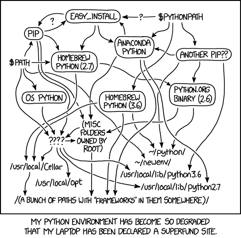
Actually, for many years, this was quite complicated, so much so that it inspired the XKCD comic below! But although there are still unfortunately many tools for reproducing Python environments, the tools and situation are much better than they once were.

It may be easier to illustrate creating Python environments with an example. Let’s say you’re using Python 3.8, statsmodels, and pandas for one project, project A. And, for project B, you’re using Python 3.8 with numpy and scikit-learn. Best practice would be to have two separate virtual Python environments: environment A, with everything needed for project A, and environment B, with everything needed for project B. This way, when you “hand over” project A to a colleague, what they need is clear—and even specified as part of the documents contained within the project. Better still, you can specify the version of Python too.

There are two ways one could create reproducible Python environments that we’re going to look at in this section: poetry and Anaconda. Poetry is recommended for full reproducibility but you may find Anaconda to be more convenient on Windows. Anaconda can get you most, but not all, of the way to reproducible Python environments and are an excellent back-up option if you don’t want to use poetry.

Before we get into the details though, a word of warning: even if you install the same packages and the same version of a programming language, you may still get differences on different operating systems (or other differences in computers, like hardware). This will be explored later on in this chapter.

Reproducible Environments with Poetry

Poetry is a relatively new but really quite amazing command line tool that performs several important tasks:

• automatically creates virtual environments on a per project basis

• manages Python package dependencies, and logs them automatically

• manages Python package versions, and logs them automatically

• installs all needed dependencies and packages from previously auto-generated (by Poetry) lists of versions

• (advanced) builds Python packages

• (advanced) uploads Python packages to PyPI where they can be installed (ie make your project pip installable)

A pre-requisite for poetry is an installation of the version of Python that you plan to use for your project.

To use poetry, install it, and navigate to your project folder within the command line. Then run poetry init. This will create a (human-readable) pyproject.toml file that lists the packages needed for your project. It will also create a virtual Python environment just for your project.

To add and install packages, the command is poetry add package-name. As you add packages, you will see that pyproject.toml automatically becomes populated with what you installed. Here’s an excerpt of a typical pyproject.toml file designed for reproducibility:

[tool.poetry.dependencies]
python = "3.7.1"
click = "8.0.1"
rich = "10.9.0"
pandas = "1.3.2"
Pygments = "2.10.0"
typeguard = "2.12.1"

The first line here says that this runs on Python 3.7.1.

A second file, poetry.lock, is also created. This “locks” down the dependencies of your packages. It’s also human-readable, just not very compelling. Visual Studio Code will happily open both types of file.

Where poetry really shines is when you send someone else the project. They receive all the files for your project, including the automatically generated pyproject.toml and poetry.lock files. Then, all they need is to have the right version of Python installed, navigate to the project folder in the command line, and enter poetry install. This will install all of the packages needed to run the code!

Note that, if you want to use the virtual environment to run scripts or tools installed using poetry add, you will need to use poetry run command-name rather than the usual command-name. For example, if you have a script analysis.py, you would call it with poetry run Python analysis.py. You can also open a command line within the virtual environment using poetry shell.

Although poetry is geared towards developers who are creating Python packages, it’s fast becoming the best go-to option for reproducible Python environments. When using poetry for reproducible research, you’re likely to want to pin to specific versions of all packages.

Semi-reproducible Environments with Anaconda

Anaconda is a package and environment manager that supports Python and R. It’s very much geared toward data science, and has been around for a while. (This book uses it for its reproducible environment.)

Note that Anaconda provides pre-built package binaries. This is especially useful on some systems where compiling packages is a nuisance (yes, it’s Windows being difficult again). For this reason, and some others to do with guarantees around package quality, Anaconda is a popular choice for corporate coding setups.

However, that doesn’t mean it’s a good choice. It has some serious failings when it comes to reproducibility, which we’ll get to.

Before we talk about reproducibility, we’re going to look at creating conda environments from a file. While creating environments from a file isn’t sufficient alone for reproducibility, it is necessary, and it’s useful to know about in any case.

Anaconda and Python environments

This section outlines a really powerful and useful feature of Anaconda that doesn’t quite get us to full reproducibility.

Anaconda has an option for creating environments from a file. It uses an environment.yml file to do this. A yaml file is just a good old text file with the extension .yml instead of .txt and a certain layout of items (human-readable). You can open and edit yaml files in Visual Studio Code. Here’s the contents of a simple environment.yml file; the packages can be pinned down just as the version of Python is (for example pandas=1.3.3 instead of pandas) but the code below just installs the latest compatible version:

name: codeforecon
channels:
  - conda-forge
dependencies:
  - python=3.8
  - pip
  - pandas
  - pip:
    - plotnine

There’s quite a bit going on here so let’s break it down. First, the version of Python. This is pinned to 3.8 by the line python=3.8. Second, the “channels” are where packages can be picked up from. “conda-forge” is a community-led effort that holds a superset of other packages and, by including it, you’re saying you’re happy for packages to come via this route too. Then the “dependencies” section lists the actual dependencies. These are what you’d get alternatively by running conda install pandas, etc., on the command line (assuming you had already installed Anaconda and put it on your computer’s PATH).

There are so many python packages out there that not all of them are available via conda or conda-forge, and sometimes the packages available on these channels are not the latest versions. So we also include pip as a dependency and then go on to say “install some dependencies via pip”, that is install these as if a person had typed pip install packagename on the command line. Remember, pip installing a package pulls it down from PyPI, which is the biggest and most widely used Python package store.

Once you have your environment.yml file, you can install it on the command line with:

conda env create -f environment.yml

It can take some time to create a new environment as Anaconda tries to resolve all possible clashes and dependencies in the packages you asked for; it takes longer the more packages you have. (As an example of an environment file that takes a really long time to solve, look no further than the one used to create this book! The book uses many packages, all with their own dependencies and constraints, to finding a set of versions that can work together is time-consuming.) To use your newly created environment, it’s

conda activate codeforecon

on the command line, where codeforecon what be whatever name you put at the start of your environment.yml file. If everything has worked you should see

(codeforecon) your-computer:your-folder your-name$

on the command line, if you’re using the bash terminal, though this book recommends the zsh terminal. Now, every time you run a command, it will be in this Python environment. You can deactivate the environment with conda deactivate to go back to the base environment or conda activate other-environment (with the name of a different existing environment) to switch.

Semi-reproducible Anaconda Python environments

Now, having delved into how Anaconda environments work, let’s think about how to make them reproducible. What we did above, pinning the version of Python but not the packages is not going to cut the mustard. Conda environment.yml files are very useful for defining desired environments but there are times, as here, when we want to be able to exactly reproduce an environment—including the dependencies of the dependencies.

Unfortunately there’s just no good way to do this with Anaconda currently. Although it’s possible to completely and automatically lock down the versions of packages installed in the first part of the environment.yml file, ie those that can be conda installed, it is not currently possible to automatically lock down the packages that are installed by pip. There are some nuances to that story, but the important point is it’s just too painful and complicated to create perfectly reproducible environments using conda & pip together right now (and, really, you want a solution that can cover both given conda doesn’t cover all Python packages).

So what do semi-reproducible Anaconda Python environments look like? They look just like what we saw above; manually creating a environment.yml with the version of Python pinned and the names of both conda and pip packages listed but without their versions. Then, to install this, it’s conda env create -f environment.yml.

Reproducible Computational Environments

“But it works on my computer!” Ever heard that? The tools in the previous section are fantastic for reproducibility but only up to a point. The hard truth is that code packages prepared for different operating systems can have differences, most often if the package contains C or other compiled language code.

For example, because it’s hard to compile code on the fly in Windows, there are pre-compiled versions of popular packages available, either through Anaconda or just on the websites of enthusiasts. The way Windows compiles code is different to Mac, which is different to Linux, and so on.

So to be really sure that your project will run exactly the same on another system, you must not only reproduce the packages and their dependencies but also the computational environment they were run in.

By far the most popular tool for creating virtual operating systems that you can then work in is called Docker. Docker containers are a “standard unit” of software that packages up code and all its dependencies so a project runs the same regardless of what your computing environment looks like. A Docker container image is a lightweight, standalone, executable package of software that includes everything needed to run an application: code, runtime, system tools, system libraries (eg the operating system) and settings. Docker essentially puts a mini standardised operating system on top of whichever one you’re using.

To run Docker, you will need to install it but be warned—it’s quite demanding on your system when it’s running.

Docker images are defined by “dockerfiles” and, as we’ve seen in the rest of this chapter, this is going to mean a plain text file with some weird formatting! Once a dockerfile is written it can then be built into an image (a time-consuming process), and finally run on your computer.

You can find lots more information about Docker on the internet, including this popular article on best practices with Docker for Python developers—although you should be aware that it is written with production-grade software in mind, not RAP.

How do you create a docker file (the text based version of your repo)? There are two main options; the former is easier but the latter comes with more guarantees about long-term reproducibility.

repo2docker

You can create a dockerfile automatically from a github repository using the repo2docker tool. repo2docker is used to create interactive repos in the supremely wonderful Binder project, which you can use to run code from this book (it’s under the rocketship icon at the top of the page).

repo2docker will look at a repository (which could be GitHub, GitLab, Zenodo, Figshare, Dataverse installations, a Git repository or a local file directory) and build a Docker container image in which the code can be executed. The image build process is based on the configuration files found in the repository.

Lots of different configuration files are supported by repo2docker. Anaconda’s environment.yml are, and it’s recommended that you export your working environment using conda env export --from-history -f environment.yml to build an image using this technology (but note that this will not pick up any packages installed using pip). Another standard option is including a requirements.txt file, which you can create from pip via pip freeze > requirements.txt.There’s an open issue in repo2docker to support poetry pyproject.toml and poetry.lock files too.

Create your own Dockerfile

Another option is to create a Dockerfile specific to your project. Here’s a simple example of a Dockerfile that loads a particular version of Python on a particular version of a Linux operating system:

# Load the Debian Linux operating system with a specific version of Python installed
FROM python:3.8.12-buster

# Update package list and install some key libraries for compiling code
RUN apt-get update && apt-get install -y gcc libffi-dev g++ libssl-dev openssl

# Ensure "python" command points to this version of Python
RUN update-alternatives --install /usr/bin/python python /usr/local/bin/python3.8 12
RUN update-alternatives --install /usr/bin/python3 python3 /usr/local/bin/python3.8 12

# ensure local python is preferred over any built-in python
ENV PATH /usr/local/bin:$PATH

# set the working directory in the container
WORKDIR /app

Of course, there’s a Visual Studio Code extension for Dockerfiles.

Note that for each instruction or command from the Dockerfile, the Docker builder generates an image layer and stacks it upon the previous ones. To make any rebuilding of your dockerfile less painful, you can ensure that only the later lines change, insofar as is possible.

To build this docker image, the command line command to run in the relevant directory is

docker build -t pythonbasic .

which will tag the built docker image with the name “pythonbasic”. To run the created image as a container, it’s

docker run -t -d --name pybasicrun pythonbasic

where --name gives the running instance a name pybasicrun. And then to enter the docker container and use commands within it, the command to launch the bash shell is

docker exec -i -t pybasicrun /bin/bash

If you run this, you should see something like:

root@ec5c6d10ebc3:/app#

Exercise

Create a Dockerfile from the above text, build it, run the container, and then jump into it. Now, inside the docker container, run printf "print('hello world')" >> test.py and then python test.py. Your “hello world” message should appear on the command line.

If you can see this, congratulations! You’ve just set up your first Python-enabled Docker container. To quit the Docker container use ctrl + c, ctrl + d.

To stop the container that’s running and remove it in one go, use docker rm pybasicrun --force once you’ve quit the running instance.

Developing using Visual Studio Code within a Docker container

Now, developing on the command line like this is no fun, clearly. You want access to all of the power of an IDE. Fortunately, Visual Studio Code is designed to be able to connect from your desktop computer to the inside of your Docker container and provide a development experience as if you were running Visual Studio Code as normal.

You can find instructions and a LOT more detail here, but the short version is that you:

1. Install the VS Code remote: containers extension (more info on that here)

2. Click on the ‘remote explorer’ icon on the left-hand panel in Visual Studio Code.

3. Select “containers” from the drop-down menu (not “SSH Targets” or “Github Codespaces”)

4. Right-click on the image you’d like to connect to (perhaps “pythonbasic” from the example above), and hit “Attach to container”

You should see a new Visual Studio Code window pop up with a message, “Starting Dev Container”. This may take a while on the first run, as VS Code installs what it needs to connect remotely. But, once it’s done, you’ll find that you can navigate your Docker container, open a terminal in it, and do a lot of what you would normally but within the Docker container.

As an aside, you can do much the same trick with other VS Code remote options—SSH or GitHub Codespaces, but don’t worry if you don’t know what these are.

Also note that you could do your entire development in a Docker container from the start if you wished to truly ensure that everything was isolated and repeatable. For extremely advanced users creating software tools, this article explains how you can create a “development container” for software development. For everyone else, a variation on what we’ve seen would be fine.

Exercise

Attach Visual Studio Code to a docker container and then use the VS Code window that is connected to your running image to create a new file called test.py. Write print('hello world') in that file, save it, and use the VS Code integrated terminal to run it within the docker container.

A docker image with poetry and all packages specified

This chapter is supposed to be about reproducibility, but we’ve taken a real detour into Docker and operating systems, and remote development. But have no fear because our digressions have been equipping us to create a fully reproducible environment.

What we need for a fully reproducible environment is the code, the language, the packages, the dependencies of the packages, and the operating system to be specified. We are now in a position to do all that. We’ll even create the DAG and pipeline using Make and graphviz!

Over at example-reproducible-research there’s a complete end-to-end example of putting all of this into practice. You can see the DAG that’s executed there, but it’s

The Dockerfile that sets up this reproducible research environment is:

# Set base image (this also loads the Debian Linux operating system)
FROM python:3.8.12-buster

# Update Linux package list and install some key libraries for compiling code
RUN apt-get update && apt-get install -y gcc libffi-dev g++ libssl-dev openssl build-essential graphviz

# Install Latex
RUN apt-get --no-install-recommends install -y texlive-latex-extra

# Ensure python points to this version of Python
RUN update-alternatives --install /usr/bin/python python /usr/local/bin/python3.8 12
RUN update-alternatives --install /usr/bin/python3 python3 /usr/local/bin/python3.8 12

# ensure local python is preferred over any built-in python
ENV PATH /usr/local/bin:$PATH

ARG YOUR_ENV

ENV YOUR_ENV=${YOUR_ENV} \
  PYTHONFAULTHANDLER=1 \
  PYTHONUNBUFFERED=1 \
  PYTHONHASHSEED=random \
  PIP_NO_CACHE_DIR=off \
  PIP_DISABLE_PIP_VERSION_CHECK=on \
  PIP_DEFAULT_TIMEOUT=100 \
  POETRY_VERSION=1.0.0

# System deps:
RUN pip install "poetry==$POETRY_VERSION"

# set the working directory in the container
WORKDIR /app

# Copy only packages to cache them in docker layer
COPY poetry.lock pyproject.toml /app/

# Install the packages
RUN poetry install $(test "$YOUR_ENV" == production && echo "--no-dev") --no-interaction --no-ansi

# Copy the current directory contents into the container at /app
COPY . /app

# Make the project
RUN poetry run make

There’s a lot going on here but mostly it’s about getting a fixed version of Python and the Debian flavour of Linux operating system, installing Latex, ensuring running python on the command line picks up the version of Python we want, installing poetry (for reproducible Python package environments), using poetry to add specific versions of packakes by installing what’s in the pyproject.toml file and poetry.lock file (neither of these are shown, but are assumed to be in the directory that is copied into the Docker container, and should have versions pinned), copying all of the contents of the current directory into the Docker container, and finally executing the DAG via poetry and make.

If you’d like to try is for yourself and execute the DAG, the instructions are: install Docker, git clone this repo, and then

1. docker build -t repro . to build an image from the Dockerfile

2. docker run -t -d --name repro_run repro to run the image

3. docker exec -i -t repro_run /bin/bash to jump into the image on the command line, or use Visual Studio Code’s remote: attach to container option.

4. To (re-run) the analysis within the container, use the command line within docker to poetry run make clean and then poetry run make.

The final output of the project, report.pdf, is saved in the outputs folder within the running docker instance.

To export the final report out of the docker container and to your current directory, use the following command on your computer (not in the container)

docker cp repro_run:app/output/report.pdf .

To exit a running Docker command line terminal, use ctrl + c, ctrl + d. To remove the image and stop it running, use docker rm repro_run --force.

Exercise

Follow the instructions in this section and export the report.pdf that’s generated from the Dockerfile.

Saving Your Analysis For Prosperity

True reproducible analysis should be findable and accessible, as well as interoperable and re-usable (these are the FAIR principles for data, but they pretty much work for analysis too). So how can you make what you’ve done findable and accessible to others?

Before we try to answer that, it’s worth noting that, for an analysis that’s to be preserved in perpetuity, you really want to freeze it in time. So although github and gitlab are great to sharing dynamically changing content, they’re not as good for long-term preservation. Or, at the very least, you need clear version labels that are used to say what version of the code was used to produce a particular analysis.

There are some fantastic options out there for preserving your code base (and therefore your reproducible project) while also making it findable and accessible. Zenodo accepts both code and data (up to 50GB at the time of writing), and gives each repo a DOI, or Digital Object Identifier, a “perma-link” that will always take users to that repository regardless of other website changes. Importantly, different versions are supported and clearly labelled.

You can also now integrate a github repo and Zenodo; instructions are available in The Turing Way.

You can also integrate Zenodo, a github repo, and Binder too: so that people coming to your analysis on Zenodo can, with a single click, create a fully interactive version of your analysis on Binder! See this blog post for details, and you may want to read the section above on repo2docker too.

Figshare is a similar service to Zenodo.

Bringing It All Together

Reproducible analysis is a bit more tricky than you thought, eh? But, as noted at the start, you can derive a lot the value by doing only some of the steps. Although it’s also worth thinking about reproducible analysis right from the start of a project so that it’s not really painful to lever it back in at the end. In research especially, because you’re exploring as you go, this can be hard work and you may have to “refactor” your code multiple times. Favouring simplicity over complexity can make it all go a lot more smoothly.

We’ve looked at numerous tools throughout this chapter, especially for reproducibility for the steps at the start from automatic execution of your RAP onwards. It’s worth suggesting a default set of tools which this book recommends as:

Recipe 1 for complete reproducible analytical pipelines

1. modular code in scripts

2. Make for automatic execution of scripts and other tools according to a directed acyclic graph

3. poetry for capturing the versions of Python, packages, and the dependencies of packages

4. manually creating a dedicated Dockerfile to reproduce an operating system

Some of these tools are not very friendly to beginners, and sometimes poetry can be less convenient for installing package dependencies that are not Python packages than conda (especially on Windows), so an alternative that goes a long way toward reproducibility is:

Recipe 2 for reproducible analytical pipelines

1. modular code in scripts

2. A “main.py” script for automatic execution of scripts and other tools according to a directed acyclic graph (Python scripts can execute terminal commands too)

3. A manually written environment.yml file for specifying the names (but not versions) of packages and the version of Python (for an example, see here)

4. creating a dedicated Dockerfile to reproduce an operating system, either manually or using repo2docker

In both cases, using a service like Zenodo to freeze your project in time, create a citation, create a DOI, and make your project findable is recommended.

Note

Use the two “recipes” above to help you decide what tools to use in your reproducible analytical pipeline.

Finally, there are a few other good programming practices that you can follow to enhance the long-term sustainability and reproducibility of your code, especially as your code base gets bigger or more complex. You may not have heard of these yet, and they will or do appear in other chapters (especially Coding and Shortcuts to Better Coding), but they are listed here for completeness.

• unit testing

• error handling

• documentation of functions via docstrings

• using a code style such as black

• consider using typing and typeguarding, at least for some code

• input data validation

• logging

• pre-commit hooks

• continuous integration