import numpy as np

a = np.array([0, 1, 2, 3], dtype="int64")
a
array([0, 1, 2, 3])In this chapter, you’ll learn about how to solve mathematical problems numerically.
If you’re running code from this chapter, remember you may need to install the packages. This chapter uses numpy, scipy, and matplotlib in particular.
Numpy arrays are the fundamental non-scalar object for numerical analysis in Python. Let’s meet a vector of integers rendered as a numpy array.
import numpy as np
a = np.array([0, 1, 2, 3], dtype="int64")
aarray([0, 1, 2, 3])Arrays are very memory efficient and fast objects that you should use in preference to lists for any heavy duty numerical operation.
To demonstrate this, let’s do a time race between lists and arrays for squaring all elements of an array:
Lists:
a_list = range(1000)
%timeit [i**2 for i in a_list]
61.2 μs ± 245 ns per loop (mean ± std. dev. of 7 runs, 10,000 loops each)Arrays:
a = np.arange(1000)
%timeit a**2
397 ns ± 4.61 ns per loop (mean ± std. dev. of 7 runs, 1,000,000 loops each)Using arrays was *two orders of magnitude** faster! Okay, so we should use arrays for numerical works. How do we make them? You can specify an array explicitly as we did above to create a vector. This manual approach works for other dimensions too:
mat = np.array([[0, 1, 2], [3, 4, 5], [6, 7, 8]])
mat
array([[0, 1, 2],
[3, 4, 5],
[6, 7, 8]])To find out about matrix properties, we use .shape
mat.shape(3, 3)We already saw how np.arange(start, stop, step) produces a vector; np.linspace(start, stop, number) produces a vector of length number by equally dividing the space between start and stop.
Three really useful arrays are np.ones(shape), for example,
np.ones((3, 3))array([[1., 1., 1.],
[1., 1., 1.],
[1., 1., 1.]])np.diag() for diagonal arrays,
np.diag(np.array([1, 2, 3, 4]))array([[1, 0, 0, 0],
[0, 2, 0, 0],
[0, 0, 3, 0],
[0, 0, 0, 4]])and np.zeros() for empty arrays:
np.zeros((2, 2))array([[0., 0.],
[0., 0.]])Random numbers are supplied by np.random.rand() for a uniform distribution in [0, 1], and np.random.randn() for numbers drawn from a standard normal distribution.
You can, of course, specify a function to create an array:
c = np.fromfunction(lambda i, j: i**2 + j**2, (4, 5))
c
array([[ 0., 1., 4., 9., 16.],
[ 1., 2., 5., 10., 17.],
[ 4., 5., 8., 13., 20.],
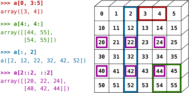
[ 9., 10., 13., 18., 25.]])To access values in an array, you can use all of the by-position slicing methods that you’ve seen already in data analysis and with lists. The figure gives an example of some common slicing operations:
Arrays can also be sliced and diced based on boolean indexing, just like a dataframe.
For example, using the array defined above, we can create a boolean array of true and false values from a condition such as c > 6 and use that to only access some elements of an array (it doesn’t have to be the same array, though it usually is):
c[c > 6]array([ 9., 16., 10., 17., 8., 13., 20., 9., 10., 13., 18., 25.])As with dataframes, arrays can be combined. The main command to remember is np.concatenate, which has an axis keyword option.
x = np.eye(3)
np.concatenate([x, x], axis=0)
array([[1., 0., 0.],
[0., 1., 0.],
[0., 0., 1.],
[1., 0., 0.],
[0., 1., 0.],
[0., 0., 1.]])Splitting is performed with np.split(array, splits, axis=), for example
np.split(x, [3], axis=0)[array([[1., 0., 0.],
[0., 1., 0.],
[0., 0., 1.]]),
array([], shape=(0, 3), dtype=float64)]Aggregation operations are very similar to those found in dataframes: x.sum(i) to sum across the ith dimension of the array; similarly for standard deviation, and so on.
As with dataframes, you can (and often should) specify the datatype of an array when you create it by passing a dtype= keyword, eg c = np.array([1, 2, 3], dtype=float). To find out the data type of an array that already exists, use c.dtype.
Finally, numpy does a lot of smart broadcasting of arrays. Broadcasting is what means that summing two arrays gives you a third array that has elements that are each the sum of the relevant elements in the two original arrays. Put another way, it’s what causes x + y = z (for arrays x and y with the same shape) to result in an array z for which z_{ij} = x_{ij} + y_{ij}.
Summing two arrays of the same shape is a pretty obvious example, but it also applies to cases that are not completely matched. For example, multiplication by a scalar is broadcast across all elements of an array:
x = np.ones(shape=(3, 3))
x * 3
array([[3., 3., 3.],
[3., 3., 3.],
[3., 3., 3.]])Similarly, numpy functions are broadcast across elements of an array:
np.exp(x)array([[2.71828183, 2.71828183, 2.71828183],
[2.71828183, 2.71828183, 2.71828183],
[2.71828183, 2.71828183, 2.71828183]])This has been the slightest introduction to arrays. For a more comprehensive overview of arrays in Python, check out the excellent “NumPy: the absolute basics for beginners” on the numpy website. If you still want more delicious arrays, check out the scipy lecture notes.
The transpose of an array x is given by x.T.
Matrix multiplication is performed using the @ operator. Here we perform $ M_{il} = {k} x{ik} * (x^T)_{kl}$, where x^T is the transpose of x.
x @ x.Tarray([[3., 3., 3.],
[3., 3., 3.],
[3., 3., 3.]])To multiply two arrays element wise, ie to do $ M_{ij} = x_{ij} y_{ij}$, it’s the usual multiplication operator *.
Inverting matrices:
a = np.random.randint(9, size=(3, 3), dtype="int")
b = a @ np.linalg.inv(a)
b
array([[1.00000000e+00, 0.00000000e+00, 2.77555756e-17],
[2.77555756e-17, 1.00000000e+00, 4.16333634e-17],
[1.11022302e-16, 0.00000000e+00, 1.00000000e+00]])Computing the trace:
b.trace()np.float64(3.0)Determinant:
np.linalg.det(a)np.float64(-229.99999999999983)Computing a Cholesky decomposition, i.e. finding lower triangular matrix C such that C C' = \Sigma for \Sigma a 2-dimensional positive definite matrix.
Σ = np.array([[4, 1], [1, 3]])
c = np.linalg.cholesky(Σ)

c @ c.T - Σ
array([[0., 0.],
[0., 0.]])Say we have a system of equations, 4x + 3y + 2z = 25, -2x + 2y + 3z = -10, and 3x -5y + 2z = -4. We can solve these three equations for the three unknowns, x, y, and z, using the solve method. First, remember that this equation can be written in matrix form as
M\cdot \vec{x} = \vec{c}
We can solve this by multiplying by the matrix inverse of M:
M^{-1} M \cdot \vec{x} = I \cdot \vec{x} = M^{-1} \cdot \vec{c}
which could be called by running x = la.inv(M).dot(c). There’s a convenience function in numpy called solve that does the same thing: here it finds the real values of the vector \vec{x}.
M = np.array([[4, 3, 2], [-2, 2, 3], [3, -5, 2]])
c = np.array([25, -10, -4])
np.linalg.solve(M, c)
array([ 5., 3., -2.])Finally, eigenvalues and eigenvectors can be found from:
import scipy.linalg as la

eigvals, eigvecs = la.eig(M)
eigvals
array([5.65662617+0.j , 1.17168692+4.51348646j,
1.17168692-4.51348646j])This section draws on the scipy documentation. There are built-in pandas methods for interpolation in dataframes, but scipy also has a range of functions for this including for univariate data interp1d, multidimensional interpolation on a grid interpn, griddata for unstructured data. Let’s see a simple example with interpolation between a regular grid of integers.
import matplotlib.pyplot as plt
from scipy import interpolate

x = np.arange(0, 10)
y = np.exp(-x / 3.0)
f = interpolate.interp1d(x, y, kind="cubic")
# Create a finer grid to interpolation function f
xnew = np.arange(0, 9, 0.1)
ynew = f(xnew)
plt.plot(x, y, "o", xnew, ynew, "-")
plt.show()
What about unstructured data? Let’s create a Cobb-Douglas function on a detailed grid but then only retain a random set of the established points.
from scipy.interpolate import griddata


def cobb_doug(x, y):
    alpha = 0.8
    return x ** (alpha) * y ** (alpha - 1)


# Take some random points of the Cobb-Douglas function
points = np.random.rand(1000, 2)
values = cobb_doug(points[:, 0], points[:, 1])

# Create a grid
grid_x, grid_y = np.mgrid[0.01:1:200j, 0.01:1:200j]

# Interpolate the points we have onto the grid
interp_data = griddata(points, values, (grid_x, grid_y), method="cubic")

# Plot results
fig, axes = plt.subplots(1, 2)
# Plot function & scatter of random points
axes[0].imshow(
    cobb_doug(grid_x, grid_y).T,
    extent=(0, 1, 0, 1),
    origin="lower",
    cmap="plasma_r",
    vmin=0,
    vmax=1,
)
axes[0].plot(points[:, 0], points[:, 1], "r.", ms=1.2)
axes[0].set_title("Original + points")
# Interpolation of random points
axes[1].imshow(
    interp_data.T, extent=(0, 1, 0, 1), origin="lower", cmap="plasma_r", vmin=0, vmax=1
)
axes[1].set_title("Cubic interpolation");
scipy has functions for minimising scalar functions, minimising multivariate functions with complex surfaces, and root-finding. Let’s see an example of finding the minimum of a scalar function.
from scipy import optimize


def f(x):
    return x**2 + 10 * np.sin(x) - 1.2


result = optimize.minimize(f, x0=0)
result
message: Optimization terminated successfully.
success: True
status: 0
fun: -9.145823375615207
x: [-1.306e+00]
nit: 5
jac: [-1.192e-06]
hess_inv: [[ 8.589e-02]]
nfev: 12
njev: 6The result of the optimisation is in the ‘x’ attribute of result. Let’s see this:
x = np.arange(-10, 10, 0.1)
fig, ax = plt.subplots()
ax.plot(x, f(x))
ax.scatter(result.x, f(result.x), s=150, color="k")
ax.set_xlabel("x")
ax.set_ylabel("f(x)", rotation=90)
plt.show()
In higher dimensions, the minimisation works in much the same way, with the same function optimize.minimize. There are a LOT of minimisation options that you can pass to the method= keyword; the default is intelligently chosen from BFGS, L-BFGS-B, or SLSQP, depending upon whether you supply constraints or bounds.
Root finding, aka solving equations of the form f(x)=0, is also catered for by scipy, through optimize.root. It works in much the same way as optimizer.minimize.
In both of these cases, be warned that multiple roots and multiple minima can be hard to detect, and you may need to carefully specify the bounds or the starting positions in order to find the root you’re looking for. Also, both of these methods can accept the Jacobian of the function you’re working with as an argument, which is likely to improve performance with some solvers.
scipy provides routines to numerically evaluate integrals in scipy.integrate, which you can find the documentation for here. Let’s see an example using the ‘vanilla’ integration method, quad(), to solve a known function between given (numerical) limits:
\displaystyle\int_0^{\pi} \sin(x) d x
from scipy.integrate import quad

res, err = quad(np.sin, 0, np.pi)
res2.0What if we just have data samples? In that case, there are several routines that perform purely numerical integration:
from scipy.integrate import simpson

x = np.arange(0, 10)
f_of_x = np.arange(0, 10)

simpson(f_of_x, x) - 9**2 / 2np.float64(0.0)Even with just 10 evenly spaced points, the composite Simpson’s rule integration given by simps is able to accurately find the answer as \left( x^2/2\right) |_{0}^{9}.
In this chapter, you should have: